Week 5 - Rayleigh Taylor Instability

Notice: - After the analysis, the size of the file is more, but in the challenge submission time it is not supported because of its large so I am sharing the google drive link please download from the link.

Link: https://drive.google.com/file/d/1Xzd2sz9yAfhaz5iafDQdAqMuAfgbT2U_/view?usp=sharing

Video link: https://drive.google.com/file/d/1jU7gxnh-KLEma2V19noOWCPu55xTfz0z/view?usp=sharing

Introduction

When the lighter fluid is pushing the heavy fluid, the Rayleigh-Taylor instability, a fingering instability at an interface between two fluids of different densities, arises. A Taylor unstable interface evolves under the influence of a complicated phenomenology. This entails the development of spikes, curtains, and bubbles as well as the growth of Helmholtz instability on the side of the spikes, competition among bubbles that results in their amalgamation, the formation of droplets, entrainment, turbulent mixing, and a potential chaotic limit with a fractalized interface.

One of the hydrodynamic instabilities that is the simplest to notice is the Rayleigh-Taylor instability. It not only causes the water to fall when we invert a glass, but it also has a significant impact on several natural processes, such as coastal upwelling, which helps replenish the nutrients near the sea's surface, and the supernova explosion that occurs when some stars reach the end of their lives. The production of some astronomical formations, such as the supernova remnants in the Eagle and Crab nebula, the formation of air bubbles in the blood of deep-sea divers, and many industrial processes all involve the Rayleigh- Taylor instability. It is a key concern in inertial confinement fusion and is also significant in plasma physics.

The mathematical analysis of Rayleigh Taylor waves has served as the foundation for certain useful CFD models, including the following.

• Saffman-Taylor Instability
• Richtmyer–Meshkov instability
• Kelvin-Helmholtz Instability
• Plateau-Rayleigh Instability

Practical models

SPH method (Smoother practice hydrodynamics)

SPH is a Lagrangian method for computing smooth field variables that are based on particle interpolation. These particles serve as control masses and carry all of the physical characteristics of the simulation system. SPH has definite advantages over conventional mesh-dependent Eulerian algorithms because of its Lagrangian character. SPH is a computational technique for modelling continuous media mechanics, including solid mechanics and fluid flows. Fluid motion is increasingly modelled with smoothed-particle hydrodynamics. This is a result of several advantages over conventional grid-based approaches. Since the particles themselves represent mass, SPH ensures the conservation of mass without the need for further calculation. Additionally, SPH computes pressure using the weighted contributions of nearby particles rather than by solving linear systems of equations.

Single fluid model

Here we use a two-phase flow mixture model analysis both fluids behave as the assumed mixture property of fluids. The five-equation applied single-fluid model consists of two equations describing the production and evolution of the liquid phase and the mass, momentum, and energy equations for a liquid mixture.

Two-fluid model

In the two-fluid model for the solution of the models two different equations are used for the fluid and different for vapour There is also no modelling of the droplet interaction or the heat transfer between the liquid phase and the solid boundary. This model also takes into account the velocity slip between the vapour and liquid phases.

Turbulence model

Inflows that are typically one or two-dimensional require the use of turbulence models to forecast the typical mixing behaviour. Experimental behaviour directs the method used to build the tile turbulence model. The equations governing turbulent flow may be directly solved only for straightforward examples of flow. Turbulence models are used in CFD simulations to forecast the evolution of turbulence for the majority of real-world turbulent flows. These turbulence models are condensed constitutive equations that forecast how turbulent flows will evolve statistically.

Modelling and solving approach

For the modelling and solving approaches, we will follow some steps

• Geometry setup
• Meshing
• Solving procedure & calculation
• Result preview

Geometry setup

In the geometry setup, we have to design the required model, in our setup, we need a 2-D model which shows two surfaces which are assigned later in two fluids. We use the shared topology for better meshing.

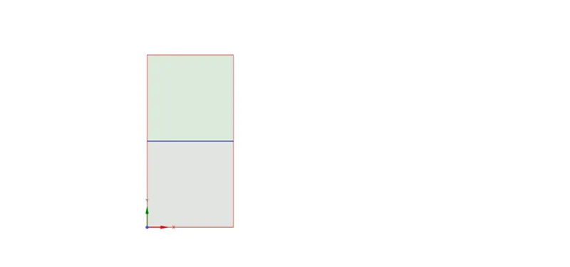
(Geometrical model)

Meshing

In our instability model, we consider two cases in the first case we consider water properties as ideal and in the second case, we change the water properties in density to 400kg/m^3 and dynamic viscosity kg/m-s. In our first case, we take the two mesh sizes of element one is 0.05mm and another one is 0.02mm.

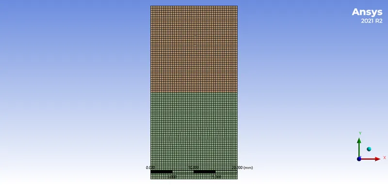
(0.05mm mesh size)

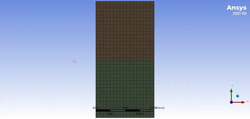
(0.02mm mesh size)

In our second case when we change the properties of the water in this condition, we consider the mesh size as 0.05mm.

Solving procedure & calculation

In both cases, we consider the same procedure for solving only in send case change in the material properties. Here we take a pressure-based solver and steady state. Give the gravitational velocity -9.81m/s^2. In the y-axis. We take the laminar flow and in multiphase define 2 phases, in the first phase we take the air and in the second phase, we take water. After hybrid initialization, we have to patch in volume fraction. After plotting a contour of the water phase, we can run the calculation.

In our second case in the material section, we change the properties of water density as 400kg/m^3 and viscosity as 0.001kg/m-s. follow the same procedure as the first case and run the calculation.

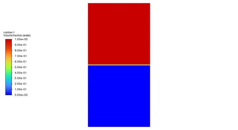
(Before the calculation)

Result

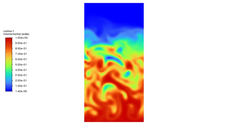
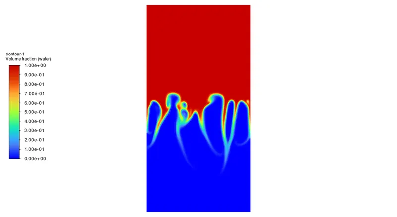
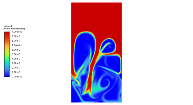
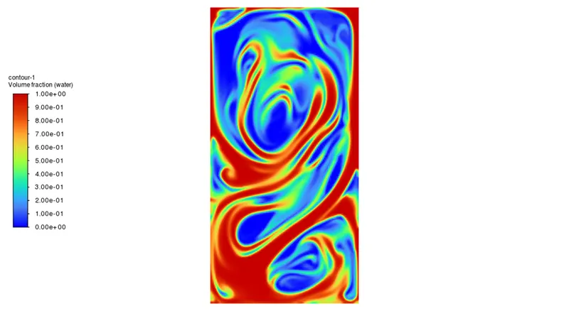
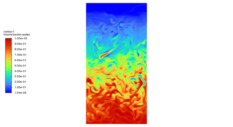
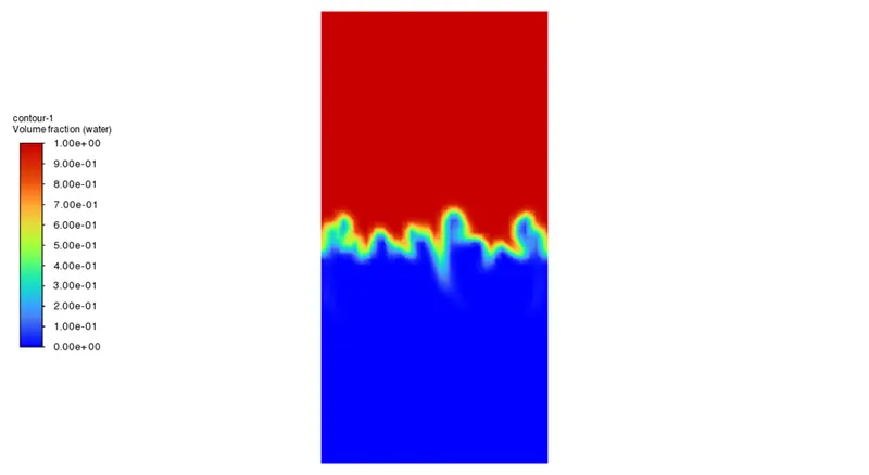
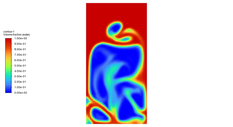
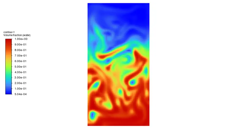
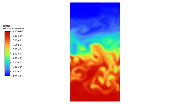
After calculation, we can see how the volume fraction will change when we change the mesh size and material properties.

Case-1

For mesh size 0.05mm

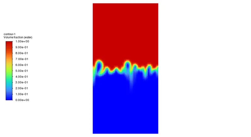
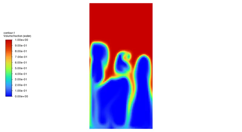
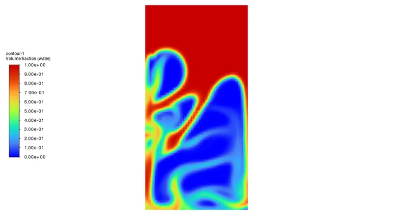
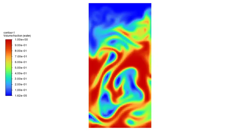
For mesh size 0.02mm

Case-2

In case 2 we change the water properties we can see the result in contour plots

Atwood Number

Fluid dynamics uses the Atwood number, a dimensionless number, to analyse hydrodynamic instability in density-stratified flows. The ratio of the difference in mass densities to their sum is known as the Atwood number.

A = {ρ(water)-ρ(air)}/ {ρ(water)+ρ(air)}

ρ(water)- Density of water

ρ(air)- Density of air

The Rayleigh-Taylor instability describes how the acceleration time scale affects the distance that heavier fluid bubbles penetrate into the lighter fluid.

Agt^2

g is the gravitational acceleration and t is the time

For case-1

ρ(water)- 997

ρ(air)- 1.225

A= (997-1.225)/ (997+1.225) = 0.9975m

For case-2

ρ(water)- 400

ρ(air)- 1.225

A = (400-1.225)/ (400+1.225) = 0.9938

From these two Atwood numbers, we can find out the penetration distance.

Conclusion

From the aforementioned examples, we can see that a finer mesh catches instability better than a coarse mesh, but that the heavier fluid takes longer to settle than a fine mesh. Despite the lengthy computing time, the results are more accurate. The transient technique is favoured over the steady-state approach because the simulation must capture instabilities that change in an unanticipated way over time. How statistically dispersed heterogeneities affect the development of instability In real-world settings, these heterogeneities are frequently present and, in some cases, have a significant impact on the flow.