Week 5 - Rayleigh Taylor Instability

AIM:

To study and analyze the rayleigh Taylor instability criterion.

OBJECTIVE:

• Perform the Rayleigh Taylor instability simulation for 2 different mesh sizes with the base mesh being 0.5 mm. Compare the results by showing the animations. Observe the differences in the animation and compare the effect of mesh size on the simulation.
• Practical CFD models have been based on the mathematical analysis of Rayleigh Taylor waves.
• Variation in Atwood number in the above two cases affects the behavior of the instability.

THEORY OF RAYLEIGH TAYLOR INSTABILITY:

Rayleigh Taylor instability was proposed by Lord rayleigh and G I Taylor states as follows which is instability between two fluids of different densities which occurs when lighter fluid is pushing the heavier fluids. For example, water lighter fluid is pushing heavier fluid. The equilibrium here is unstable to any perturbations or disturbances of the interface: if a parcel of heavier fluid is displaced downward with an equal volume of lighter fluid displaced upwards, the potential energy of the configuration is lower than the initial state. Thus the disturbance will grow and lead to a further release of potential energy, as the more dense material moves down under the (effective) gravitational field, and the less dense material is further displaced upwards.

MULTIPHASE flow is a simulation(parallel) flow of materials with different states or phases(liquid-gas). It is a flow of materials with different chemical properties but in the same state or phase(liquid-liquid)

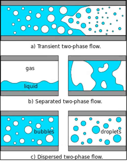
TYPES OF PHASES IN MULTIPHASE

1. Separated phase- is defined as one or more immiscible fluids in a continuous phase separated by an interface.
2. mixed phase- is defined as the phase in which one or more fluids are mixed together. this phase contains both separate and dispersed phases
3. dispersed phase- is the phase in which the finite number of phases are spread in the continuous phase.

VOLUME OF FLUID(VOF)

The volume of fluid method is the surface tracking method. It is designed to determine the interface's position between two or more immiscible fluids. The volume fraction of each fluid in each cell throughout the domain can be tracked by using this method. A single set of momentum is shared only by the fluids. In this method, all the control volumes must be filled with a single phase or combination of phases.

Application of the VOF model includes stratified flows, free surface flows, filling, sloshing, the motion of larger bubbles in liquids, steady or transient tracking of any liquid-gas interface, prediction of jet breakup(surface tension), and the motion of liquid in the dam break.

Some practical CFD models have been based on the mathematical analysis of Rayleigh Taylor waves and these mathematical models have been adapted for CFD calculations

1. Kelvin-Helmholtz instability
2. Richtmyer-Meshkov instability
3. Plateau-Rayleigh instability

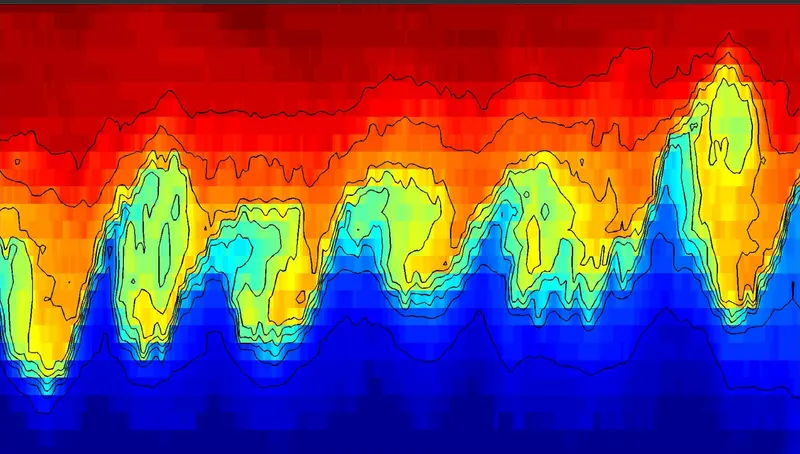
Kelvin-Helmholtz instability- This instability typically occurs when there is velocity shear in a single continuous fluid, or additionally where there is a velocity difference across the interface between two fluids. A common example is seen when the wind blows across a water surface. The below images for KH are shown 500m deep in the Atlantic ocean.

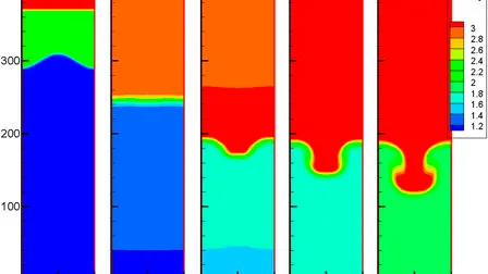
Richtmyer-Meshkov instability- This occurs when two fluids of different densities are impulsively accelerated. Normally this is by the passage of a shock wave. The development of the instability begins with small amplitude perturbations which initially grow linearly with time. A nonlinear regime follows this with bubbles appearing in the case of a light fluid penetrating a heavy fluid, and spikes appearing in the case of a heavy fluid penetrating a light fluid. A chaotic regime eventually is reached and the two fluids mix. This instability can be considered the impulsive-acceleration limit of the Rayleigh Taylor instability.

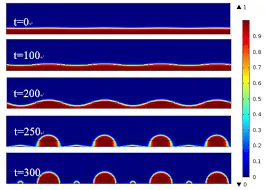
Plateau-Rayleigh instability- This instability, often just called the Rayleigh instability, explains why and how a falling stream of fluid breaks up into smaller packets with the same volume but less surface area. It is related to the RTI and is part of a greater branch of fluid dynamics concerned with fluid thread breakup. This fluid instability is exploited in designing a particular type of inkjet technology whereby a jet of liquid is perturbed into a steady stream of droplets. The driving force of the Plateau–Rayleigh instability is that liquids, by virtue of their surface tension, tend to minimize their surface area.

DETAILED PROCEDURE FOR SIMULATION OF RAYLEIGH TAYLOR INSTABILITY USING ANSYS FLUENT

In this report, we are going to study separate phases using ANSYS fluent where for the first case study I am considering water and air due to instability between the water and air separated layers since the water has a high density(we are not considering additional force but here we are gravitational force(g=9.81m^2/s). Due to density differences, the water and air are going to mix causing instability this case is studied using the ANSYS tool. Similarly, in case 2 is studied instead of using air we are going to perform user-defined values(density = 400 kg/m³, viscosity = 0.001 kg/m-s) and study the instability criteria.

GEOMETRY

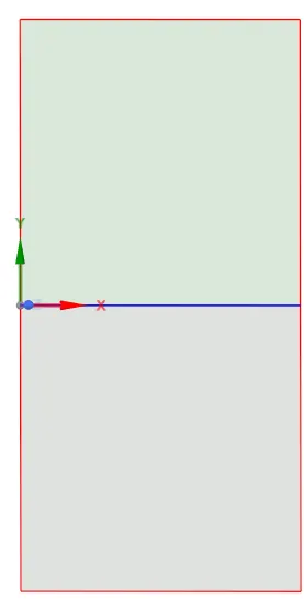
• The geometry is essentially two squares, one on top of another on a side of 20 mm. The top square has been named 'water' and the bottom square 'air'.
• The common edge between the domains was shared using the share tool in Workbench. The created geometry is shown below. Hence under the WORKBENCH=> select the SHARE option.

MESH

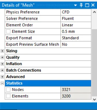
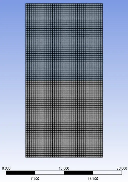
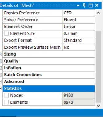
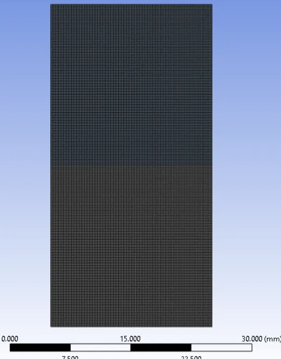
Meshing is based on the element size of 3 cases as shown below.

case 1:

Mesh properties

Element size=0.5mm

case 1:

Mesh properties

Element size=0.3mm

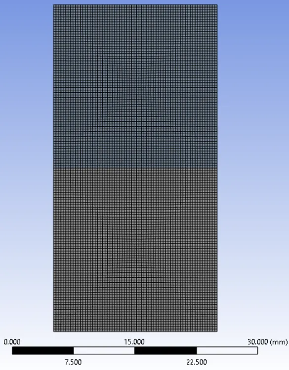
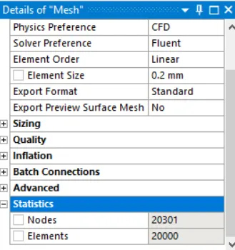
Mesh properties

Element size=0.2mm

SETUP AND SOLUTION

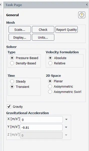
• Initially, we go for the SOLVER option here we are the type of solver used is PRESSURE BASED SOLVER (M<0.3), enable GRAVITY with y=-9.81, and since the variable is varying with respect to time select the TRANSIENT STATE option.
• In the following step in for the PHYSICS, the window selects the VISCOUS option we get the window opened up. Here we select the LAMINAR flow model.

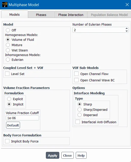
• In the multiphase model, we are enabling VOF homogeneous model with implicit parameters.

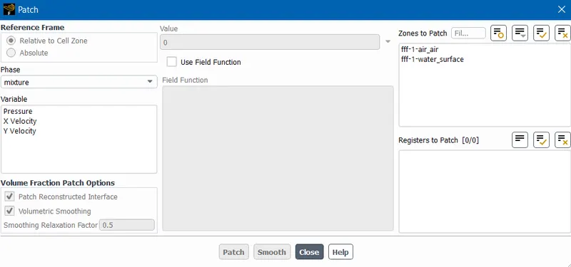
• In the PATCH option in order to differentiate the scale plotted in contour for the water surface, we have to patch both the domains to the respective materials, wherein we provide a volume-fraction value of 1 to water and 0 to air and user-defined material.

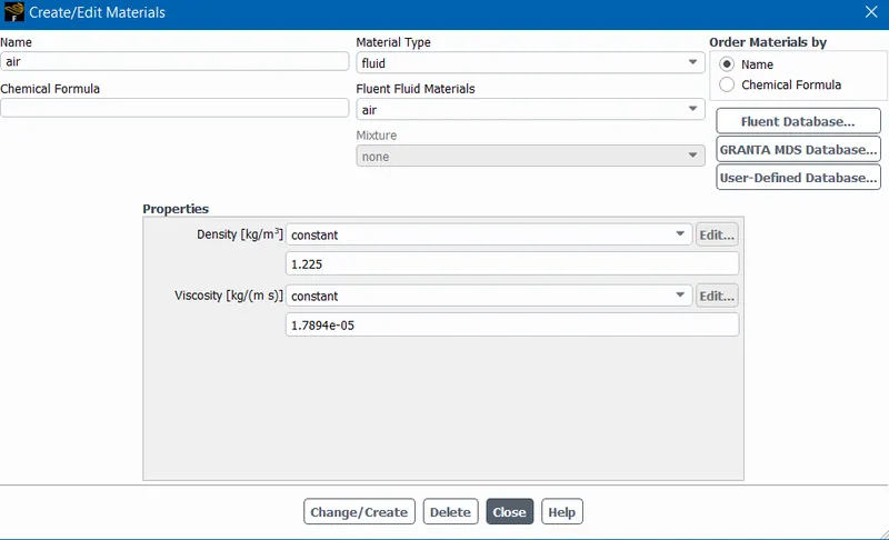
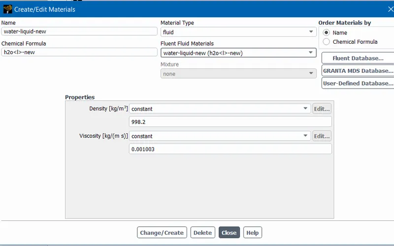
After solving for a number of Time steps(500) with 0.001 dt (time step size), the following solution/animation was obtained:

Case 1: Element size=0.5mm

Case 2: Element size=0.3mm

Case 3: Element size=0.2mm

Case 4: a mesh of 0.2m with user-defined properties

Atwood number

It is a dimensionless number that is used to study hydrodynamic instabilities in density stratified flows. Atwood number is an important parameter in the study of Rayleigh-Taylor instability. For Atwood numbers close to 0, RT instability flows take the form of asymmetric “finger” of fluid; for Atwood numbers close to 1, the much lighter fluid “below” the heavier fluid takes the form of larger bubble-like plumes. The calculated Atwood number is close to 1 and from the simulation results, it is found that when high dense fluid i.e. water poured upon low dense fluid i.e. air under gravity, the formation of air bubble-like plumes takes place which travels towards the upward region in the form of waves and some gets trapped at the lower regions during the initial stages, which afterward try to move towards the upper region and at the end, both phases gets separated with some diffusivity left at the middle portion between them.

`A=(rho1-rho2)/(rho1+rho2)`

`rho1`is the density of a heavier fluid

`rho2` is the density of a lighter fluid

For Air-water RT instability,

`rho1`= 998 `(kg/(m^3)`water density

`rho2`= 1.22 `(kg/(m^3)`air density

`A=(998-1.22)/(998+1.22)`

A=0.9875

For water- UD material RT instability

`rho1`= 998 `(kg/(m^3)`water density

`rho2`= 400 `(kg/(m^3)`air density

`A=(998-400)/(998+400)`

A=0.420

Atwood number affects the behavior of the instability

• When the Atwood number is close to 1, the much lighter fluid below the heavier fluid takes the form of larger bubbles like plumes.
• For Atwood numbers close to 0, RT instability flows take the form of symmetric figures of fluid.
• Therefore, from the value of the Atwood number, it is seen from the simulations that air forms larger bubbles when water is poured down the air pushes through and forms large bubbles. Therefore, the results can be validated by obtaining the value of the Atwood number. Atwood number is an important parameter in the body of Rayleigh Taylor's instability.

CONCLUSIONS:

• Since the simulation involves capturing instabilities that are changing in an unpredictable manner as a function of time, the transient approach is preferred over the steady-state approach.
• Finer mesh captures the instability better than the coarse mesh, but it takes more time for the heavier fluid to settle down. So it is computationally expensive but produces results with better accuracy.