Week 3 - Solving second order ODEs

AIM:

Write a program in MATLAB that solves Second-order ordinary differential equations(ODE) for the simple pendulum with damping and also to simulate the pendulum's motion for given input variables to the simple pendulum with respect to time.

THEORY:

A simple pendulum consists of a Ball of mass(m) hanging from a string of length of L and which is fixed at a pivot point. When the bob is held at an initial angle and released, the pendulum swings back and forth with the periodic motion. Since it is periodic motion there involves both angular displacement and angular velocity with respect to different positions of the Ball.

The motion of the pendulum depends on Newton's Second Law, When this law is written down, we get Second order ODE's that describes the position of the Ball with respect to time.

Ordinary differential equations(ODE) is a differential equation containing one or more functions of one independent variable and other derivates of those functions. In the above simple pendulum, we are coding in order to determine the angular displacement and angular velocity for various angles of the ball with respect to the fixed surface by using second-order ODE we get the required solution for a given input. MATLAB uses the ODE45 command to solve ODE related problems.

GOVERNING EQUATIONS:

SECOND-ORDER ODE

`frac{partial ^2 theta}{partial t^2}+frac{b}{m}frac{partial theta}{partial t}+frac{g}{l]sintheta=0`

Where b is damping coefficient (constant), m is mass of the ball in (kg), g is gravity in (m/s^2), L is length of the pendulum in (m).

CONVERTING HIGHER ORDER ODE's INTO FIRST ORDER ODE's

`frac{partial^2 theta}{partial t^2}+frac{b}{m} frac{partial theta}{partial t}+frac{g}{l}sintheta=0`

In the above second-order ode should be converted into first-order ode by subtitution method [`theta`=`theta1`]

`theta`=`theta1`

`frac{partial theta}{partial t}=frac{partial theta1}{partial t}=theta2`

`frac{partial^2theta}{partial t^2}=frac{partial}{partialt}(frac{partial theta1}{partialt})=frac{partial}{partial t}(theta2)`

`frac{partial theta1}{partialt}=theta2`

`frac{partial theta2}{partialt}=-frac{b}{m}theta2-frac{g}{l}sintheta1`

`frac{partial}{partialt}[frac{theta1}{theta2}]=[frac{theta2}{-frac{b}{m}theta2-frac{g}{l}sintheta1}]`

MATLAB CODE:

clear all
close all
clc

%initial conditions for b,g,l,m, angular displacement and angular velocity
b=0.05;
g=9.81;
l=1;
m=1;
theta_0=[0;3];

%Time period
t_span=linspace(0,20,200);

%Solving 2nd order ODE by using ode45 command
[t,results]=ode45(@(t,theta) ode_func1(t,theta,b,g,l,m),t_span,theta_0);

%graph of angular dissplacement and angular velocity
figure(1)
plot(t,results);
legend('angular displacement','angular velocity');

%Animation of motion of pendulum
figure(2)
ct=1;
 %FOR loop is used inorder to get each frame of pendulum from obtained 'results' data
 for i=1:length(results(:,1))
     x0=0;
     y0=0;
     %Calculation of position of ball with respect to (x0,y0) which is (x1,y1) 
     x1=l*sin(results(i,1));
     y1=-l*cos(results(i,1));
     
     %Plotting the simple pendulum 
     plot([-1 1],[0 0],'linewidth',4,'color','b')
     hold on
     plot([0 0],[0.5 -1.5],'linewidth',2,'linestyle','--')
     hold on
     plot([x0 x1],[y0 y1],'linewidth',4,'color','g')
     hold on
     plot(x1,y1,'o','MarkerSize',20,'markerfacecolor','r')
     hold off
     axis ([-1.5 1.5 -1.5 0.5]);
     pause(0.02);
     %Storing each frame in array called 'M'
     M(ct)=getframe(gcf);
     ct=ct+1;
 end
 %Creating a movie document by adding each frame obtained from above array of 'M'
 movie(M)
 videofile=VideoWriter('ode4.avi','uncompressed AVI');
 open(videofile)
 writeVideo(videofile,M)
 close(videofile)

Subprogram using FUNCTION command

function [dtheta_dt]=ode_func1(t,theta,b,g,l,m)

theta1=theta(1);
theta2=theta(2);
dtheta1_dt=theta2;
dtheta2_dt=-(b/m)*theta2-(g/l)*sin(theta1);
dtheta_dt=[dtheta1_dt;dtheta2_dt]
end

CODE EXPLANATION:

1. The first step of Matlab programming is to make sure when the new file is opened all the variables, plots, and command windows must be cleared by using (clear all, close all, clc)commands.
2. Basic input variables such as b, g, l, m, and also angular displacement and angular velocity at time t=0 are assigned.
3. 'linspace' command is used for equal distribution of time period for the calculation of ODE.
4. In order to calculate angular displacement and angular velocity associated with different positions made by the ball, the ode45 command is used.
5. Function command 'ode_func1' is used to ease our programming code to look tedious and also for calculation dtheta1_dt, dtheta2_dt. These above variables are returned when the function is called in the main programming as shown in the above code.
6. Once we get an array of elements containing angular displacement and angular velocity, we proceed with further steps to create an animation of a simple pendulum.
7. FOR loop is used to access each and every frame created for the simple pendulum for different values of angle with respect to a fixed surface.
8. (x1,y1) is the point at which the ball is represented for each angle/movement of the pendulum[y1 is negative because of the pendulum is oscillated in 3rd and 4th quadrants].
9. Plot command is used to create each line associated with the pendulum diagram as shown above code.
10. Marker command is used to create a ball with appropriate size and color.
11. Once the simple pendulum diagram for each value of theta is stored in an array called M by using a command called 'GetFrame' command.
12. In this final step, all the images of a simple pendulum are stored in an array known as M, and its stitched to make a movie by using 'videoWriter' command[to create uncompressed avi], 'open' command[to open videofile], 'Writevideo' command[to add all the images stored in array M to be stitched into a movie], 'Close' command[to close the video file.

ERRORS:

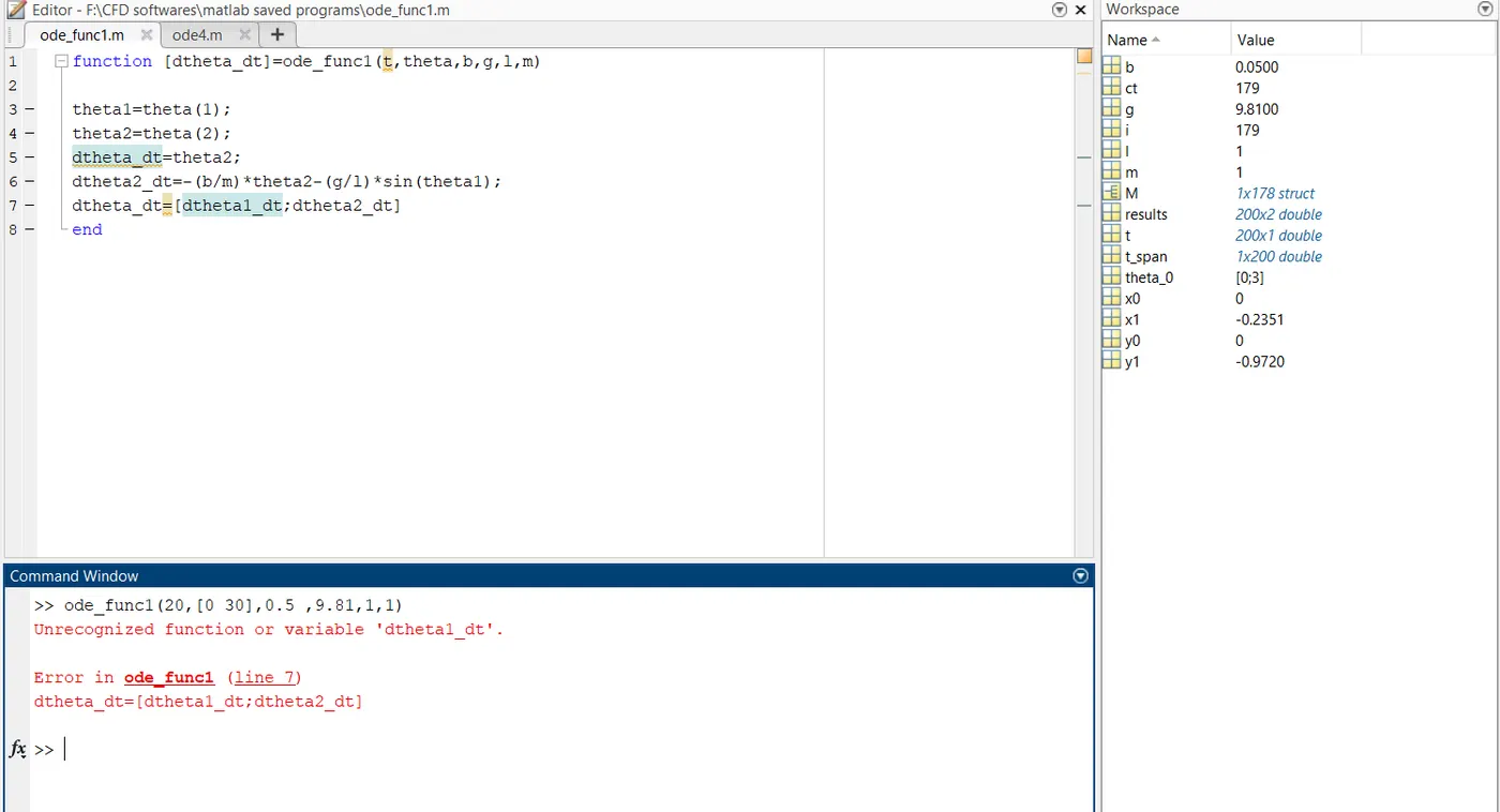
The above error has occurred in the function subprogram(ode_fun1) which is due to the wrong representation of variable 'dtheta1_dt', Hence it is been rectified.

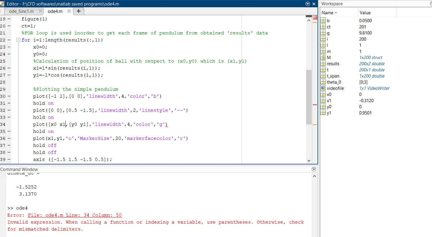
The above error is due to the missing a square bracket in the plot command i.e[x0,y0], Hence it is been rectified.

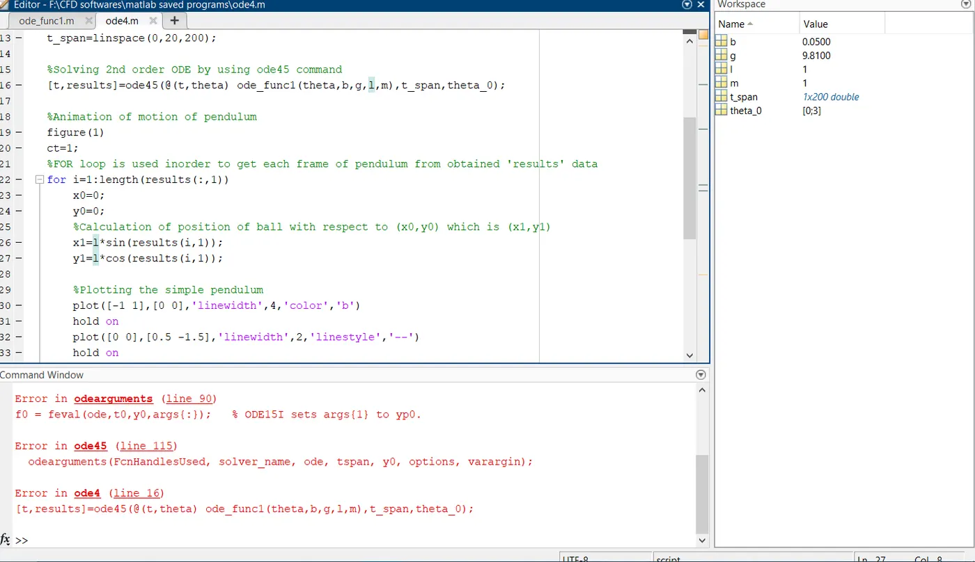
The above error has occurred due to missing a variable 't' in the 'ode45' command, Hence it is been rectified.

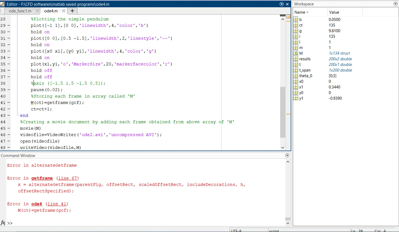
The above errors occur when the program has been executed multiple times, due to this there is the repetitive replacement of images in an array called M. Hence it is been rectified.

RESULTS:

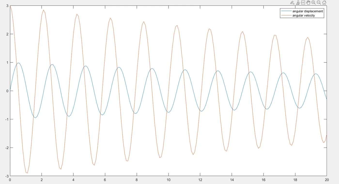
Angular displacement vs Angular velocity.

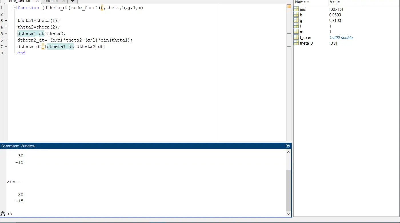
When the function program 'ode_func1' is executed we get the above results which are displayed in the command window.

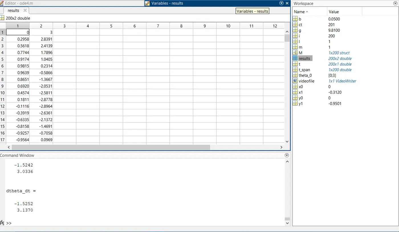
The above program is executed for obtaining the results of both angular displacement and angular velocity by using the 'ODE45' command as displayed in the table.

ANIMATION/OSCILLATION OF SIMPLE PENDULUM

https://drive.google.com/file/d/1YiNfvNDiMLxqJb5pZ6ZubVyzE64bkTIp/view?usp=sharing

CONCLUSION:

Hence the angular displacement and angular velocity of the simple pendulum for different positions of the ball are displayed and also the animated video of the simple pendulum has been presented through the above link.