Week 4.1 - Genetic Algorithm

AIM:

Write a MATLAB code to optimize the given stalagmite function by using a genetic algorithm. Finally, we are finding global maxima for a given stalagmite function using boundary conditions.

THEORY:

OPTIMIZATION

Optimization is an area of study which deals with how to minimize or maximize the particular function which depends on multiple input parameters (or) optimization refers to finding input values in such a way that we get the desired "best output" values. In this MATLAB code, we are using the stalagmite function for optimization to get global maxima.

For a given problem the optimization is performed based on input variables, constraints, and objective function. The set of all possible values which the input can take make up the search space. In this search space, lies a point or set of points that gives the optimal solution. Optimization aims to find that point or set of points in the search space.

GENETIC ALGORITHM

A genetic algorithm(GA) is a method of solving both constrained and unconstrained optimization problems based on the natural selection process that mimics biological evolution. This algorithm repeatedly modifies the population of the individual solutions until the sequence of points approaches the optimal solution.

In a genetic algorithm, we have a population of solutions to a given problem. These solutions undergo recombination and mutation(natural genetics), producing new hybrids and this is repeated over generations. Each solution is assigned a fitness value based on its objective function value and the fitter individual are given a higher chance to mate and yield more fitter individuals. In this way, we keep evolving better individuals over generations, till we reach a stopping criterion.

Genetic algorithms are sufficiently randomized in nature, but they perform much better than random local search( in which we just try various random solutions, keeping track of the best so far), as they exploit the information as well.

PROCESS OF NATURAL SELECTION

The process of natural selection starts with the selection of the fittest individual from the population. They produce offsprings who inherit the characteristics of the parents which is added to the next generations. If the parents have better fitness, their offspring will be better than their parents and have a better chance of surviving. This process keeps on iterating and in the end, a generation with the fittest individuals will be found. This notation can be applied to the search problem. we consider a set of solutions for a problem and select the best ones out of them.

Five phases are considered in the genetic algorithm

1. Initial population
2. Fitness function
3. Selection
4. Crossover
5. Mutation

• Initial population- The process begins with a set of individuals which is called a population. Each individual is a solution to the problem you want to solve and an individual is characterized by a set of parameters(variables) known as Genes. Genes are joined into a string to form a chromosome(solutions). In a genetic algorithm, the set of genes of an individual is represented using a string in terms of an alphabet. Usually, binary values are used.

• Fitness function(Evaluation function)- evaluates how close a given solution is to the optimum solution of the desired problem. The reason behind using the fitness function is in a genetic algorithm, each solution is generally represented as a string of binary numbers known as a chromosome. We have to test these solutions and come up with the best set of solutions to solve a given problem. Each solution, therefore, needs to be awarded a fitness score to indicate how close it came to meeting the overall specification of the desired solution. This score is generated by applying the fitness function to the test or results obtained from the tested solution.

• Selection- The selection is based on the fitness score. The idea of the selection phase is to select the fittest individuals and let them pass their genes to the next generation. Two pairs of these individuals(parents) are selected based on their fitness scores. Individuals with high fitness have more chances to be selected for reproduction.

• Crossover- Crossover is the most significant phase in a genetic algorithm. For each pair of parents to be mated, a crossover point is chosen at random from within the genes. Offspring are created by exchanging the genes of parents among themselves until the crossover point is reached.

• Mutation- In certain new offspring formed, some of the genes can be subjected to a mutation with a low random probability. This implies that some of the bits in the bit string can be flipped. The mutation occurs to maintain diversity within the population and prevent premature convergence. The algorithm terminates if the population has converged does not produce offspring which are significantly different from the previous generation.

Then it is said that the genetic algorithm has provided a set of solutions to our problem. The population has fixed size as new generations are formed, individuals with the least fitness die, providing space for new offspring. The sequence of phases is repeated to produce individuals in each new generation who are better than the previous generation. GA as a function of MATLAB.

STALAGMITE FUNCTION

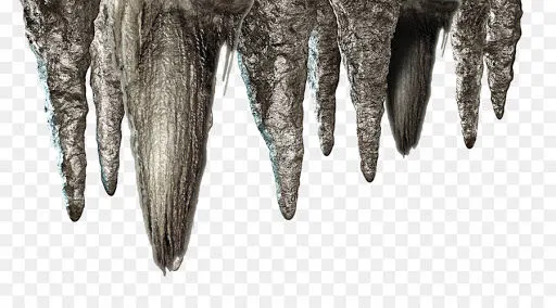
Stalagmite is an upward growing mound of mineral deposits that have precipitated from water dripping onto the floor of the cave.

A stalagmite function refers to the function with which we are generating values over a stalagmite kind of surface for finding out the local and global maxima and minima of that particularly given function.

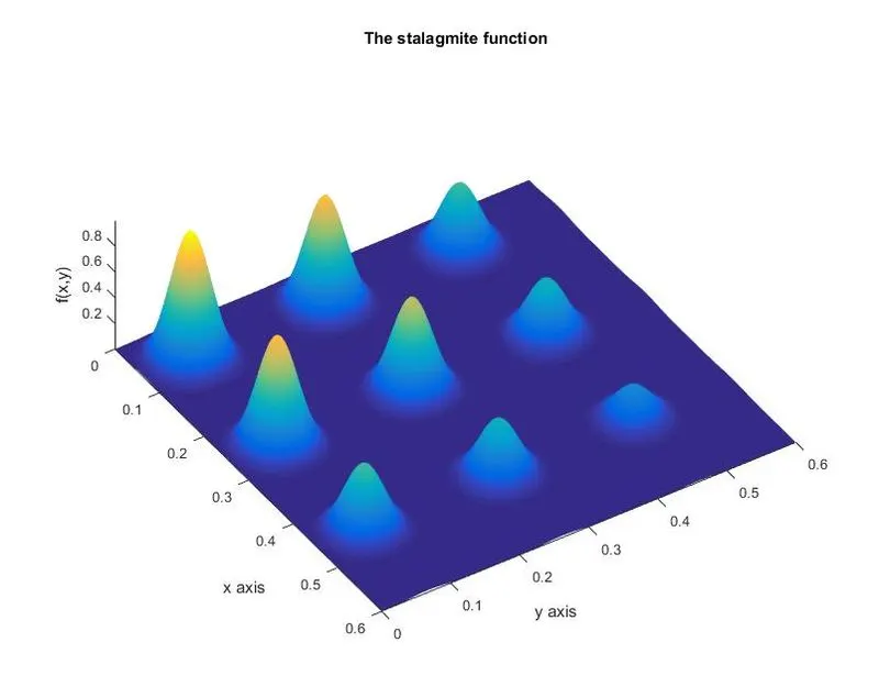
GOVERNING EQUATIONS:

SYNTAX FOR GENETIC ALGORITHM

1. `x=ga(fun,nvars)`

`x=ga(fun,nvars)` finds a local unconstrained minimum of x to the objective function(func) for nvars(number of design variables) of func.

2. `x=ga(fun,nvars,A,B)`

`x=ga(fun,nvars,A,B)`finds local minimum of x to func, subjects to the linear inequalities A*x<=b. Evaluates the matrix product A*x as if x is transposed(A*x').

3. `x=ga(fun,nvars,A,B,Aeq,Beq)`

`x=ga(fun,nvars,A,B,Aeq,Beq)` finds local minimum of x to fun, subjects to liner equations Aeq*x=Beq and A*x<=B. Set A=[ ] and B=[ ] if no linear inequalities exist, ga evaluates the matrix product Aeq*x as if x is transposed (Aeq*x').

4.`x=ga(fun,nvars,A,B,Aeq,Beq,lb,ub)`

`x=ga(fun,nvars,A,B,Aeq,Beq,lb,ub)` defines a set of lower and upper bounds on the design variables, x, so that a solution is found in the range lb<= x <= ub (Set Aeq=[ ] and Beq=[ ] if no linear equalities exist.

5. `x=ga(fun,nvars,A,B,Aeq,Beq,lb,ub,nonlcon)`

`x=ga(fun,nvars,A,B,Aeq,Beq,lb,ub,nonlcon)` subjects the minimization to the constraints defined in nonlcon. The function NONLcon accepts x and returns vectors C and Ceq, representing the nonlinear inequalities and equalities respectively. ga minimizes the fun such that C(x) <= 0 and Ceq=0.

6. `x=ga(fun,nvars,A,B,Aeq,Beq,lb,ub,nonlcon,options)`

`x=ga(fun,nvars,A,B,Aeq,Beq,lb,ub,nonlcon,options)` minimizes with the default optimization parameters replaced by values in 'options'. (Set nonlcon=[ ] if no nonlinear constraints exist). Create options using optimoptions.

7. `[x,fval]=ga( )`

`[x,fval]=ga( )`for any previous input arguments also returns fval, the value of the fitness function at x.

MATLAB CODE:

clear all
close all
clc

%creating values for x and y using linspace command
x=linspace(0,0.6,150);
y=linspace(0,0.6,150);
numcase=50;

%creating 2D array
[xx,yy]=meshgrid(x,y);

%For given values of [xx,yy] we are creating stalagmite function
for i=1: length(xx)
    for j=1:length(yy)
        input_vector(1)= xx(i,j);
        input_vector(2)= yy(i,j);
        f(i,j)= stalagmite1(input_vector);
    end
end
 
 %Study1-unbounded case
 tic
 for i=1:numcase
     [results,fopt(i)]=ga(@stalagmite1,2);
     xopt(i)=results(1);
     yopt(i)=results(2);
 end
 study1=toc;
 figure(1)
 subplot(2,1,1);
 surf(x,y,-f);
 shading interp
 hold on
 plot3(xopt,yopt,-fopt,'marker','o');
 subplot(2,1,2);
 plot(-fopt);
 xlabel('iterations');
 ylabel('function maximum')
 disp(study1);
 
 %Study2-Bounded case
 tic
   for i=1:numcase
      [results,fopt1(i)]=ga(@stalagmite1,2,[],[],[],[],[0;0],[0.6;0.6]);
          xopt1(i)=results(1);
          yopt1(i)=results(2);
   end
 study2=toc;
 figure(2)
 subplot(2,1,1);
 surf(x,y,-f);
 shading interp
 hold on
 plot3(xopt1,yopt1,-fopt1,'marker','o');
 subplot(2,1,2);
 plot(-fopt1);
 xlabel('iterations');
 ylabel('function maximum');
 disp(study2);
 
 %Increased population size
 tic
 options=optimoptions('ga');
 options=optimoptions(options,'populationsize',250);
   for i=1:numcase
      [results,fopt2(i)]=ga(@stalagmite1,2,[],[],[],[],[0;0],[0.6;0.6],[],[],options);
          xopt2(i)=results(1);
          yopt2(i)=results(2);
   end
 study3=toc;   
 figure(3)
 subplot(2,1,1);
 surf(x,y,-f);
 shading interp
 hold on
 plot3(xopt2,yopt2,-fopt2,'marker','o');
 subplot(2,1,2);
 plot(-fopt2);
 xlabel('iterations');
 ylabel('function maximum');
 disp(study3);

STALAGMITE FUNCTION CODE

function[D] = stalagmite1(input_vector)
x=input_vector(1);
y=input_vector(2);
f1=(sin(5.1*pi*x+0.5))^6;
f2=(sin(5.1*pi*y+0.5))^6;
f3=exp(-4*log(2)*((x-0.0667)^2/0.64));
f4=exp(-4*log(2)*((y-0.0667)^2/0.64));
D=-(f1*f2*f3*f4);
end

CODE EXPLANATION:

1. The first step in MATLAB programming is to make sure when a new file is opened all the variables and command windows must be cleared by using (clear all, close all, and clc) commands.
2. Before starting the MATLAB code we should make sure the stalagmite1 function code and main code should be saved in the same folder.
3. First, we initialize the values of x and y taking 150 values between the intervals 0 and 0.6. Also, we consider the number of iterations(numcase) to be 50.
4. For getting a Two-Dimension array of elements containing values of x and y we use the meshgrid command.
5. Since we need a three-dimensional plot we take the two-dimensional array values of x & y and store them in an input-vector array, so that it can be used as an argument to call the function stalagmite1.
6. We create another function code file for the stalagmite function(Stalagmite1) and we here take the output as -f since GA only minimizes a given function. if -f is considered it automatically gives us the maxima.
7. The first study is to consider the unbounded case where we take the number of iterations equal to numcase and we genetic algorithm function to calculate the maxima of the function. We store the output into results that contain maxima's and fopt which contain the value at which the maxima is obtained. Here the GA is initiated with the random population.
8. In this step, we store the results into xopt, yopt and now we need to plot the surface of x,y,-f to get the 3D plot. we use the plot3 command to make a plot of xopt, yopt, and -fopt to plot the optimum maxima's. Also, let us plot the fopt function so that we can visualize the optimum values at each iteration. In order to get the Time taken to complete the cycle, we use the tic toc command to record the time.
9. The second study is to consider the bounded case where we specify lower and upper bounds of x and y. In this case, GA is initiated with a random population.
10. Now in this Bounded case, we store the results into xopt, yopt and we need to plot the surface of x, y, -f to get the 3D plot. We use the plot3 command to make a plot of xopt, yopt, and -fopt to plot the optimum maxima's. Also, let us plot the fopt function so that we can visualize the optimum values at each iteration.
11. The third study is to consider the initial population and bounded value. In this case, let increase our initial population which is default 50 to 250. Here the initial population is set by using the command called optimumoptions and get our value of 'populationsize' to 250. Now we store the results into xopt, yopt and we need to plot the surface of x, y, and -f to get the 3D plot.
12. We use the Plot3 command to make a plot of xopt, yopt, and -fopt to plot the optimum maxima's. Also, let us plot the fopt so that we can visualize the optimum values at each iteration.

ERRORS:

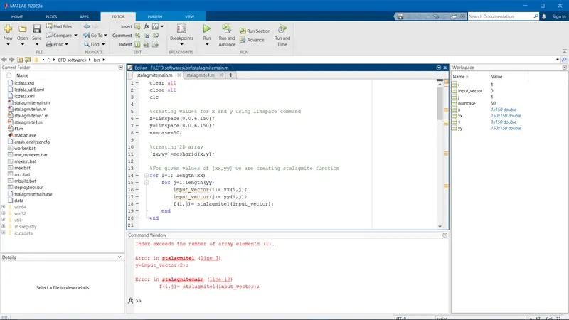
The above error has occurred due to the wrong usage of input_vector(i) & input_vector(j) inside the FOR loop in order to plot the stalagmite function hence its rectified by using column number 1 and 2 which is input_vector(1) and input_vector(2).

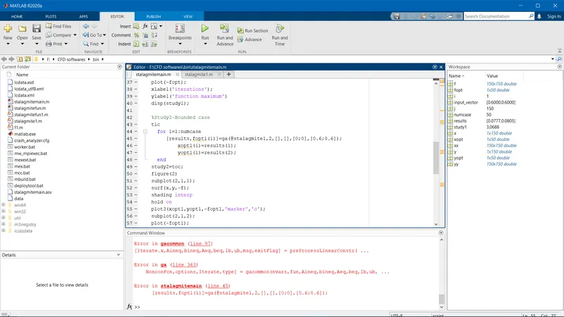
The above error has occurred due to not using the null vector(In bounded case for linear equalities), Hence its rectified by including the null vector.

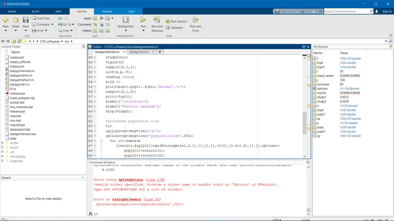
The above error has occurred due to not using 'options' in the study for population-size hence it's rectified by mentioning this variable.

RESULTS:

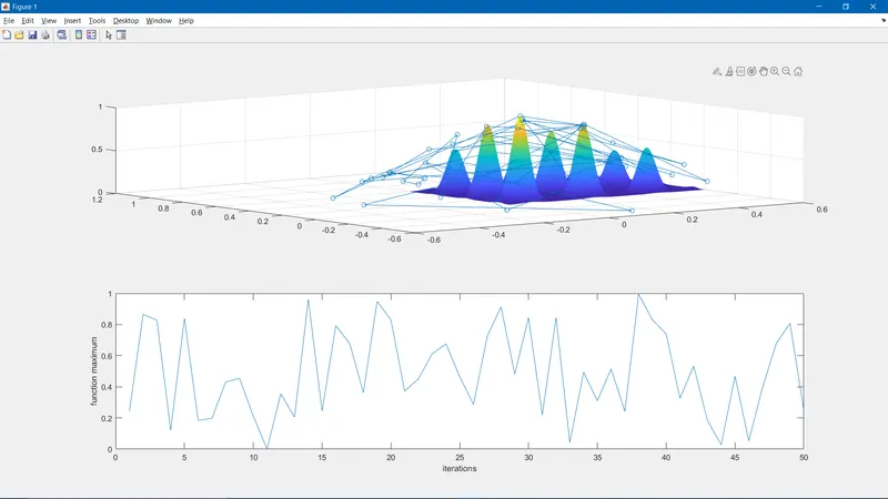
For the unbounded case, Here we can see the optimum values went outside the values of x and y resulting in falling away from the stalagmite surface. Hence we failed to reach the global maxima in this case.

Study time=2.7949s.

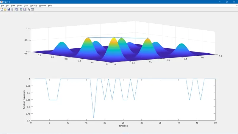
For the Bounded case, Here we can see through the optimum values are within the limits it could not give us the exact maxima values.

Study time=3.5269s.

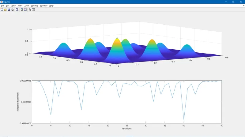
For the third study with initial population and bounded values, Here in this we successfully find out the correct maxima for the given stalagmite function(though the execution time is more). So by increasing the initial population size of GA we can increase the accuracy of the algorithm.

Study time=12.6765s.

The Global maxima point is located at(x,y,z) which is ( 0.06683,0.06683,1).

CONCLUSION:

Hence we study for all three cases and see as the population size varies the global maxima vary but in the third case study as the initial population size is increased then the accuracy of the algorithm is increased to find the global maxima. Hence the Global maxima point is at (0.06683,0.06683,1).