Project 2 - Rankine cycle Simulator

Aim:

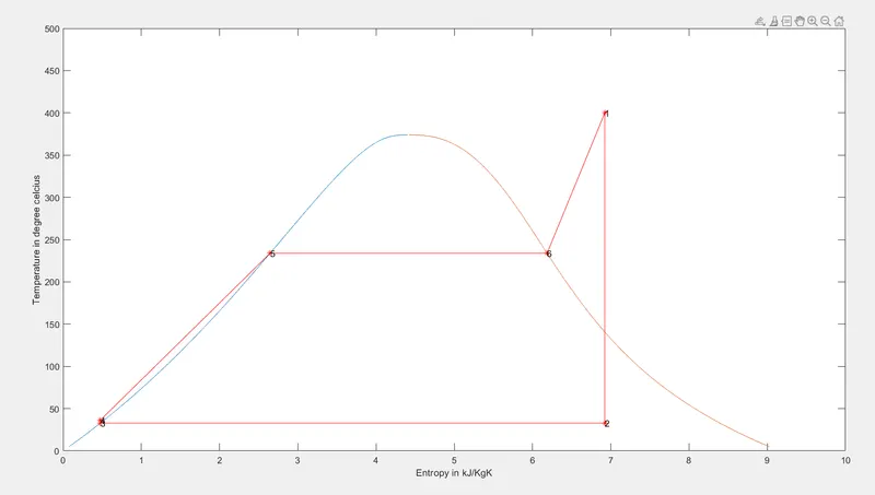
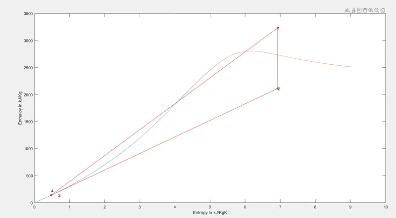
Write a MATLAB code to create a Rankine cycle simulator to calculate the parameters at each state point based on given user input values also to plot T-S and H-S diagrams.

OBJECTIVE:

• Initially, we write a program to calculate the parameters(Temperature, Pressure, Enthalpy, Entropy) at each state point.

• In this stage, we add thermodynamic relation for getting state points in between the variables.

• Finally, we plot the Rankine cycle on T-S and H-S curves.

THEORY:

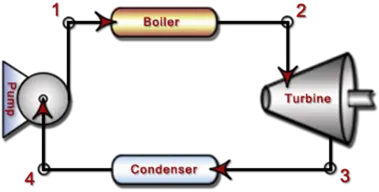
RANKINE CYCLE is an idealized thermodynamic cycle that describes the process of heat engines such as steam turbine which allows mechanical work to be extracted from a fluid as it moves between the heat source and heat sink. This cycle was named after Willam John Macquorn Rankine who was a Scottish polymath professor at Glasgow University. In this thermodynamic cycle working fluid used is water because it has various properties such as Good thermal properties, non-reactive, highly abundant, low cost. This simulator consists of a Boiler, Turbine, condenser, and pump. The Mechanical power which is obtained is dependent on the temperature difference between a heat source and a heat sink(Higher the temperature difference more the Power can be taken out from the system).

TYPES OF RANKINE CYCLE

1. Reheat Rankine cycle
2. Regenerative Rankine cycle
3. Organic Rankine cycle
4. Supercritical Rankine cycle

In the above MATLAB code, we use IDEAL RANKINE CYCLE. This operates slightly different from than Real Rankine cycle, Ideal Rankine cycle is a "Reversible cycle" where common sources of irreversibilities are neglected such as frictional pressure drops and undesired heat transfer to the surroundings. In this Rankine cycle, the Isobaric process and Isentropic Process are used to evaluate the above process to get standard results.

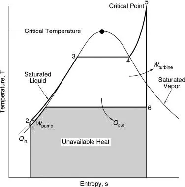
To get an Idealized Rankine cycle we need four processes which are:

• Process 1-2: Turbine[Iscentropic Expansion]

The turbine contains series of stationary and moving blades. Using the steam work is generated through the expansion of vapor which indeed is converted into electricity through the generator. This process is Iscentropic expansion because entropy remains constant whereas temperature and pressure decrease.

• Process 2-3: Condenser[Isobaric Heat rejection]

Since steam is already exhausted now to recover exhaust steam from the turbine hence we convert steam into the water using a condenser. The condenser consists of tubes that accommodate the heat transfer of steam and cooling water where the cooling water is a separate stream. The quality of fluid changes until it reaches a saturated liquid state due to this Entropy decreases by maintaining constant pressure.

• Process 3-4: Pump[Iscentropic compression]

The Pump's main purpose is to convey condensed steam[water] back into the boiler. Work is needed to pump the water back into the boiler. Since there is work involved equipment we assume this to be an isentropic process where entropy is constant and temperature slightly increases.

• Process 4-1: Boiler[Isobaric Heat transfer]

High-pressure fluid is pumped back into the boiler where the water is converted into saturated steam or superheated steam. This is an Isobaric process where pressure is kept constant where temperature and entropy increase.

GOVERNING EQUATIONS:

• Work done by Turbine

`W_t=h1-h2`

where W_t is work done(J), h is Enthalpy at that state(kJ/kg).

• Work done by Pump

`W_p=h4-h3`

where W_P is work done(J), h is Enthalpy at that state(kJ/kg).

• Net work done

`WNet=W_t-W_p`

• Heat supplied

`q=h1-h4`

• Efficiency

`n=(WNet)/q`

• Specific steatm consumption(SSC)

`SSC=3600/(WNet)`

• Dryness fraction

`S2=SL2+(x2*SLV2)`

We simplify the above equation to get x2

`x2=(S2-SL2)/(SV2*SL2)`

• XSteam function is an inbuilt Matlab function that is used to access the steam table parameters such as temperature, pressure, Enthalpy, and Entropy.

Syntax: variable_name=XSteam('condition',input1,input2)

• Heat capacity ratio(c)

`c=(Cp)/(Cv)`

MATLAB CODE:

clear all
close all
clc
 
 disp('                                                          RANKINE CYCLE SIMULATOR                         ');
 disp(' ');
 disp('Process 1-2 is iscentropic expansion in Turbine');
 disp('Process 2-3 is Constant Pressure Rejection in Condenser');
 disp('Process 3-4 is iscentropic compression in Pump');
 disp('Process 4-1 is Constant Pressure Heat addition in Boiler');
 disp(' ');
 
%Input parameters

 disp('Enter the inputs for pressure and temperature');
 disp(' ');
 T1=input('Enter the Temperature at turbine inlet(degree C):');
 p1=input('Enter the Pressure at turbine inlet(bar):');
 p2=input('Enter the Pressure at condenser inlet(in degree C:');
 
 
%Calculating Enthalpy, Entropy at state point1[Turbine inlet]
Tsat=XSteam('Tsat_p',p1);
h1= XSteam('h_pT',p1,T1);
S1=XSteam('s_pT',p1,T1);

%Calculating Enthalpy, Entropy at state point2[condenser inlet]
%Iscentropic Expansion
S2=S1;
SL2=XSteam('sL_p',p2); %Entropy of Liquid
SV2=XSteam('sV_p',p2); %Entropy of Vapour
    
%Dryness Fraction(x2)
%S2=SL2+(x2*SLV2)
x2=(S2-SL2)/(SV2-SL2);
T2=XSteam('T_ps',p2,S2);
h2=XSteam('h_px',p2,x2);
hL2=XSteam('hL_p',p2);

%Calculating Pressure,Temperature,Enthalpy,Entropy at state point3[Pump inlet]
%Constant Pressure removal process
p3=p2;
T3=T2;
S3=SL2;
h3=hL2;

%Calculating Pressure,Temperature, Enthalpy, Entropy at state point4[Boiler input]
S4=S3;
p4=p1;
h4=XSteam('h_ps',p4,S4);
cp=XSteam('cp_ps',p4,S4); %specific heat 
cv=XSteam('cv_ps',p4,S4); %specific volume
c=cp/cv;
T4=T3*((p4/p3)^(c-1)/c);

%State points 5,6 parameters
h5=XSteam('hL_p',p1);
S5=XSteam('sL_p',p1);
T5=XSteam('T_hs',h5,S5);
h6=XSteam('hV_p',p1);
S6=XSteam('sV_p',p1);
T6=XSteam('T_hs',h6,S6);


%Calculating Work done by the Turbine
W_t=h1-h2;

%Calculating Work done by Pump
W_p=h4-h3;

%Net work done
W_net=W_t-W_p;

%Heat supplied
q=h1-h4;

%Thermal Efficiency
n=(W_net/q)*100;

%Specfic heat consumption
ssc=3600/W_net;

%Displaying the each state points parameters
disp(' ');
disp('The following are results of rankine Cycle simulation');
disp(' ');
disp('At State Point 1 ');
c1=sprintf('P1 is : %.2f bar',p1);
disp(c1);
c2=sprintf('T1 is : %.2f deg celcius',T1);
disp(c2);
c3=sprintf('H1 is : %.2f kj/kg',h1);
disp(c3);
c4=sprintf('S1 is : %.2f kj/kgK',S1);
disp(c4);


disp(' ');
disp('At State Point 2 ');
c5=sprintf('P2 is : %.2f bar',p2);
disp(c5);
c6=sprintf('T2 is : %.2f deg celcius',T2);
disp(c6);
c7=sprintf('H2 is : %.2f kj/kg',h2);
disp(c7);
c8=sprintf('S2 is : %.2f kj/kgK',S2);
disp(c8);  
c9=sprintf('x2 is : %.2f kj/kgK',x2);
disp(c9);

disp(' ');
disp('At State Point 3 ');
c10=sprintf('P3 is : %.2f bar',p3);
disp(c10);
c11=sprintf('T3 is : %.2f deg celcius',T3);
disp(c11);
c12=sprintf('H3 is : %.2f kj/kg',h3);
disp(c12);
c13=sprintf('S3 is : %.2f kj/kgK',S3);
disp(c13);  

disp(' ');
disp('At State Point 4 ');
c14=sprintf('P4 is : %.2f bar',p4);
disp(c14);
c15=sprintf('T4 is : %.2f deg celcius',T4);
disp(c15);
c16=sprintf('H4 is : %.2f kj/kg',h4);
disp(c16);
c17=sprintf('S4 is : %.2f kj/kgK',S4);
disp(c17);
disp(' ');
c18=sprintf('Wt is : %.2f J',W_t);
disp(c18);
c19=sprintf('Wp is : %.2f J',W_p);
disp(c19);
c20=sprintf('Wnet is : %.2f J',W_net);
disp(c20);
c21=sprintf('Efficiency(n) is : %.2f percent ',n);
disp(c21);
c22=sprintf('SSC is : %.2f kg/kWh',ssc);
disp(c22);

%plotting T-S diagram
t=linspace(5,400,25000);
for i=1:length(t)
    s(i)=XSteam('sL_t',t(i));
     S(i)=XSteam('sV_t',t(i));
      h(i)=XSteam('hL_t',t(i));
       H(i)=XSteam('hV_t',t(i));
end
%Plotting the T-S curve
figure(1)
plot(s,t);
hold on
plot(S,t);

%plotting state points
plot([S1,S2],[T1,T2],'marker','*','color','r');
text(S1,T1,'1');
plot([S2,S3],[T2,T3],'marker','*','color','r');
text(S2,T2,'2');
plot([S3,S4],[T3,T4],'marker','*','color','r');
text(S3,T3,'3');
plot([S4,S5],[T4,T5],'marker','*','color','r');
text(S4,T4,'4');
plot([S5,S6],[T5,T6],'marker','*','color','r');
text(S5,T5,'5');
plot([S6,S1],[T6,T1],'marker','*','color','r');
text(S6,T6,'6');
axis([0,10,0,500]);
xlabel('Entropy in kJ/KgK');
ylabel('Temperature in degree celcius');

%Plotting H-S diagram
figure(2)
plot(s,h);
hold on
plot(S,H);
plot([S1,S2],[h1,h2],'marker','*','color','r');
text(S1,h1,'1');
plot([S2,S3],[h2,h3],'marker','*','color','r');
text(S2,h2,'2');
plot([S3,S4],[h3,h4],'marker','*','color','r');
text(S3+0.2,h3,'3');
plot([S4,S1],[h4,h1],'marker','*','color','r');
text(S4,h4+80,'4');
axis([0,10,0,3500]);
xlabel('Entropy in kJ/KgK');
ylabel('Enthalpy in kJ/Kg');

CODE EXPLANATION:

1. The first step of MATLAB programming is to make sure when a new file is opened all the variables and command windows must be cleared by using(clear all, close all, clc).
2. By using the disp command we display all necessary statements i.e(Rankine simulator) onto the command window and also we input the values from the user for pressure and temperature by using the input command.
3. Once we input the values of temperature and pressure values we start to calculate Entropy and enthalpy values at state point 1 by using the 'XSteam' function.
4. For state point 2 since it is an Isentropic process(S2=S1) entropy of liquid and gas is found by XSteam. Once entropy is found dryness fraction is found by using the above formula, this dryness fraction is used to calculate the enthalpy and temperature values.
5. At state point 3(Pump) since it is a constant pressure removal process pressure, temperature, entropy, enthalpy are calculated as shown in the above code.
6. At state point 4(Boiler) Cp and Cv values are found using the XSteam function in order to obtain the Heat capacity ratio. This heat capacity ratio value is used to calculate the temperature(T4).
7. Enthalpy, Entropy, and temperature are found at state points 5,6 in order to plot the points in the T-S graph.
8. Based on the obtained values of Enthalpy, Entropy at each state point, Work done by turbine and work done by pump is calculated. Finally, Net-work done is calculated.
9. Similarly in the next step, we find out heat supply, Thermal efficiency, Specific Steam consumption is calculated.
10. Based on the above-obtained values of State points parameters, values are displayed in a systematic order by using both sprintf and disp command.
11. Following step wherein we are plotting T-S diagram. Initially, we are using the linspace command to get the N number of divisions of temperature values which is used in FOR loop to create an array of elements containing the values of enthalpy and entropy of both liquid and vapor state. These array values are used to plot the T-S and H-S diagrams.
12. Finally, to connect the state points we use a plot command to connect two points and mark the point by using the 'marker' option. Text command is used to label the respective State points.

ERRORS:

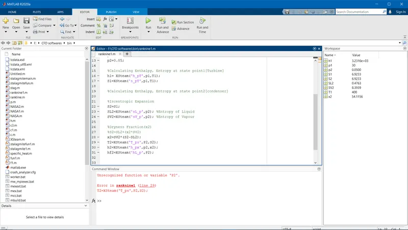
The below error has occurred due to the wrong notation of the P2 variable. Hence it is rectified.

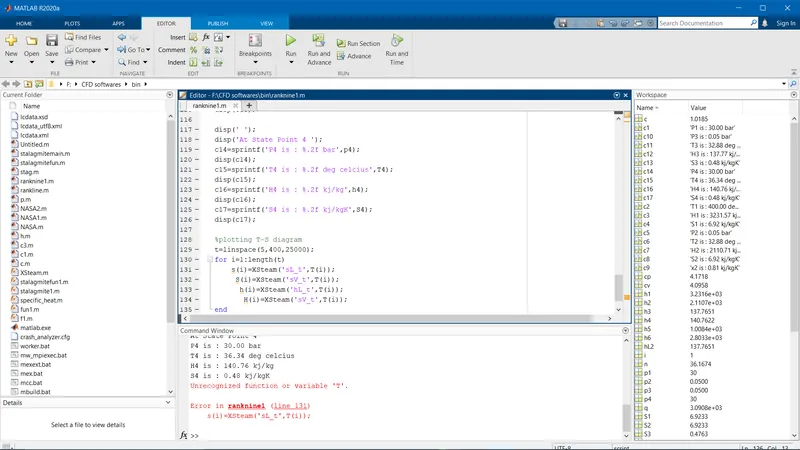
The below error has occurred due to not using the appropriate variable for Temperature inside the FOR loop. Hence it is rectified.

RESULTS:

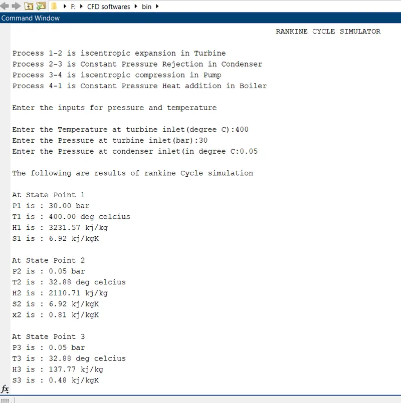
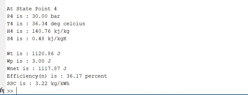
This is the output for the Rankine cycle simulator which is displayed in the command window as shown below.

T-S DIAGRAM:

H-S DIAGRAM:

CONCLUSION:

From the above Rankine cycle MATLAB code, we calculate various state point parameters such Enthalpy, Entropy, Pressure, Temperature, thermal efficiency, Work done(turbine and pump), SSC and display them in the command window also plot T-S and H-S diagrams as shown in the result section.