Week 5 - Rayleigh Taylor Instability
Aim: To study the Rayleigh Taylor Instability effect in CFD
Objective:
- What are some practical CFD models that have been based on the mathematical analysis of Rayleigh Taylor waves? In your own words, explain how these mathematical models have been adapted for CFD calculations.
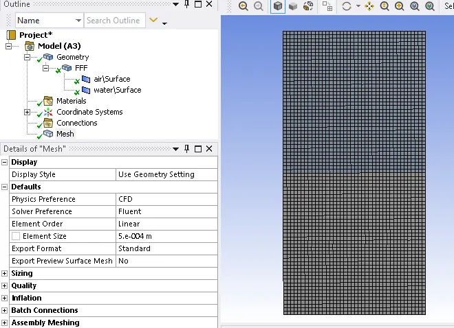
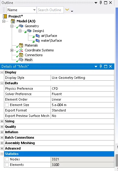
- Perform the Rayleigh Taylor instability simulation for 2 different mesh sizes with the base mesh being 0.5 mm. Compare the results by showing the animations( Attach them from your google drive). Observe the differences in the animation and explain the effect of mesh size on simulation. Also, explain why a steady-state approach might not be suitable for these types of simulation.[ Choose Air and Water for this simulation]
- Run one more simulation with water and user-defined material(density = 400 kg/m3, viscosity = 0.001 kg/m-s) for refined mesh.
- Define the Atwood Number. Find out the Atwood number for both the cases and explain how the variation in Atwood number in the above two cases affects the behavior of the instability.
What are some practical CFD models that have been based on the mathematical analysis of Rayleigh Taylor waves? In your own words, explain how these mathematical models have been adapted for CFD calculations
Richtmyer–Meshkov instability (RMI):
The Richtmyer–Meshkov instability (RMI)occurs when two fluids of different density are impulsively accelerated. Normally this is by the passage of a shock wave. The development of the instability begins with small amplitude perturbations which initially grow linearly with time. This is followed by a nonlinear regime with bubbles appearing in the case of a light fluid penetrating a heavy fluid, and with spikes appearing in the case of a heavy fluid penetrating a light fluid. A chaotic regime eventually is reached and the two fluids mix. This instability can be considered the impulsive-acceleration limit of the Rayleigh-Taylor-Instability.
Plateau–Rayleigh instability:
The Plateau–Rayleigh instability, often just called the Rayleigh instability, explains why and how a falling stream of fluid breaks up into smaller packets with the same volume but less surface area. It is related to the Rayleigh-Taylor Instability and is part of a greater branch of fluid dynamics concerned with fluid thread breakup. This fluid instability is exploited in the design of a particular type of ink jet technology whereby a jet of liquid is perturbed into a steady stream of droplets.
The driving force of the Plateau–Rayleigh instability is that liquids, by virtue of their surface tension, tend to minimize their surface area. A considerable amount of work has been done recently on the final pinching profile by attacking it with self-similar solutions
The Kelvin–Helmholtz instability:
The Kelvin–Helmholtz instability is a fluid instability that occurs when there is velocity shear in a single continous fluid or a velocity difference across the interface between two fluids. Kelvin-Helmholtz instabilities are visible in the atmosphere of planets and moons, such as in cloud formation on Earth or the Red Spot on Jupiter, and the atmosphere of the sun and other stars.
Some Pratical application:
Water Channel:
Motivated by shear-flow experiments of Brown and Roshko [95], a flow channel type setup for generating an RT unstable interface was pioneered by Snider and Andrews [96]; the experiment consisted of two parallel coflowing streams (cold and hot water) initially separated by a thin plate (see Fig. 9(a), henceforth referred to as the WC). Two 500-gallon tanks fed water to the facility; the cold-water stream was fed on top-stream, and warm water was fed into the lower-stream. The cold and warm water streams entered the channel at a mean velocity of ∼4.4 cm/s, thereby eliminating any shear (KHI) roll-ups. For the flow channel configuration, the distance downstream (x) is converted to time, t = x/U, using Taylor's hypothesis [97,98]. The flow-channel configuration allows for long data-collection times and is significantly easier to diagnose than the transient experiments. The density difference was achieved through a temperature difference of 5–10 °C in water. Temperature data were collected through a thermocouple system and converted to density through an equation of state [99]. After termination of the splitter plate, the resulting flow configuration was RT unstable, and a mixing layer develops downstream. Various diagnostics have been developed over the last decade which includes: (a) optical techniques to measure the volume fraction profiles and the growth of the mixing layer (see Fig. 9(b)); (b) high-resolution thermocouples and PIV/PLIF [100] (PIV) to investigate the velocity and density fluctuations within the mixing layer and the degree of molecular mixing within the layer (see Fig. 9(c)) [47,48,101,102]. Besides, detailed turbulence statistics, which include measurements of density and velocity variance (energy) spectra [47,102], Reynolds stress tensor at various downstream locations; and statistics of a high Schmidt number reacting mixing layer [103] has also been measured. The facility was also used to study the combined effects of buoyancy and shear at small Atwood numbers [101,104] and a buoyant plane wake [105]. However, due to the usage of hot- and cold-water as the two fluids, the WC facility is limited to a maximum Atwood number of ∼10−3
Gas Channel:
To address the Atwood number limitation of WC, a gas channel facility that uses air and helium as the two streams was subsequently developed [46,106–108] at Texas A&M (henceforth referred to as GC1). Two gas streams, one containing air and the other a helium–air mixture, flow parallel to each other separated by a thin splitter plate. The streams meet at the termination of the splitter plate leading to the formation of RTI induced mixing (see Fig. 10(a)). Like the WC experiment, the gas channel allowed for long data collection times and was statistically steady. The facility design allows for large Atwood number studies (up to At ∼ 0.75). The flow was diagnosed using backlight imaging techniques and hot-wire anemometry. Two hot-wire anemometry techniques were developed to measure a variety of turbulence statistics in the air-helium RTI mixing layer. The first diagnostic used a multiposition, multi-overheat (MPMO) single-wire technique. A single-wire response function was estimated to variations in density, velocity, and orientation; the method provides time-averaged statistics but was restricted to moderate At < 0.25. The second diagnostic works on the concept of temperature as a fluid marker. It uses a four-wire configuration; a simultaneous three-wire/cold-wire anemometry technique (S3WCA) was developed to measure instantaneous statistics. Both methods were validated in a low Atwood number (At ≤ 0.04) by comparing various statistics with PIV measurements in the water channel facility. Good agreement was found for the measured growth parameters, velocity fluctuation anisotropy, probability density function (PDF) and molecular mix parameters. The techniques were then used to measure density and velocity statistics using both regular and conditional averaging methods in a large Atwood number RT mixing layers (At ∼ 0.6) [46,108–110]. Asymmetries in the mixing layer were observed at the high Atwood number experiments (At > 0.45), Fig. 10(b) shows a snapshot of an At ∼ 0.6 experiment. A similar coflowing system with improved features and the ability to explore Reynolds numbers beyond the mixing transition threshold [20,111,112] was subsequently built at Georgia Tech to study RTI mixing at high Atwood numbers At > 0.5 (see Fig. 10(c), henceforth referred to as GC2). The GC2 facility has been designed with the option to perform multilayer experiments. Visualization and Mie-scattering techniques were implemented to obtain volume fraction profiles and mix-widths. Asymmetry was evident in the flow field, with the spike side of the mixing layer growing 50% faster than the bubble side [50]. PIV was implemented for the first time in these high-Atwood-number experiments to obtain velocity and density statistics across the mixing layer. Besides, the dynamics of the coupled shear (KHI) and RTI has also been explored in recent experiments [113]. The flow was governed by KHI dynamics at early times and RTI dynamics at late times with the transition from KHI to RTI dynamics occurring at Richardson number [Ri =−2ghAt/(ΔU)2=−2ghAt/(ΔU)2] range of 0.17–0.56.
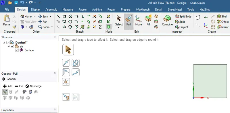
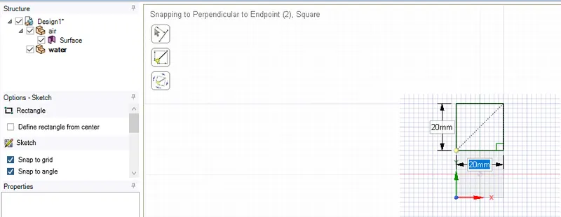
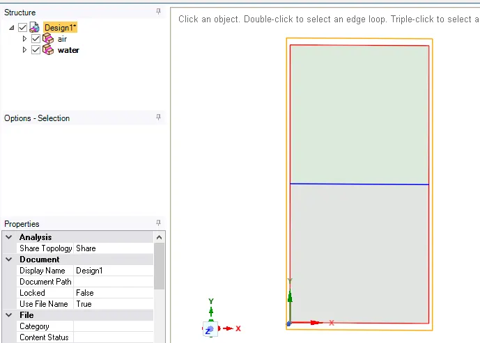
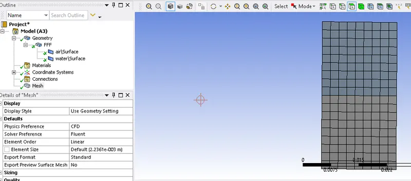
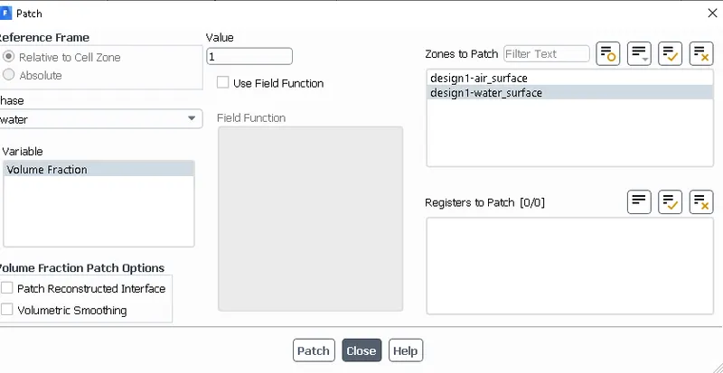
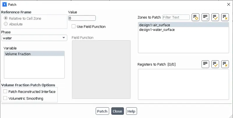
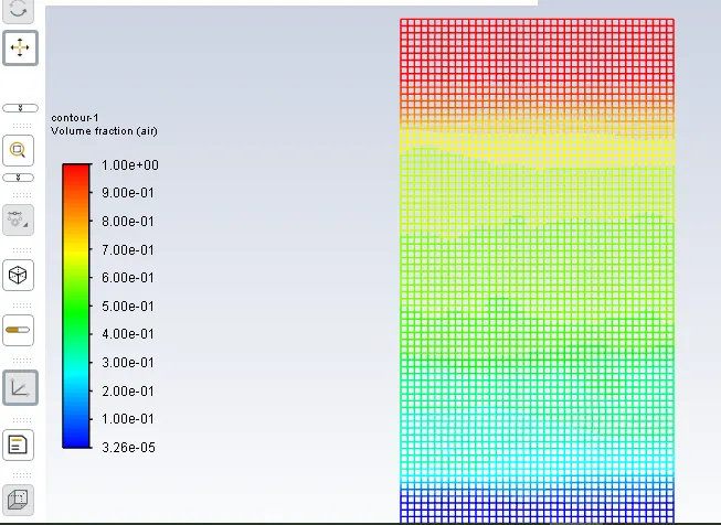
Animation Link:
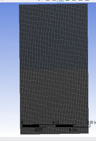
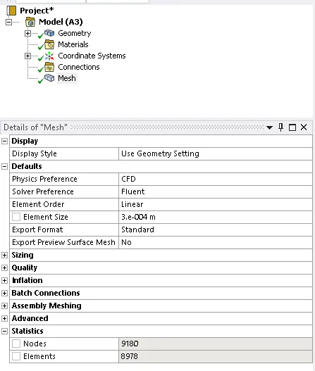
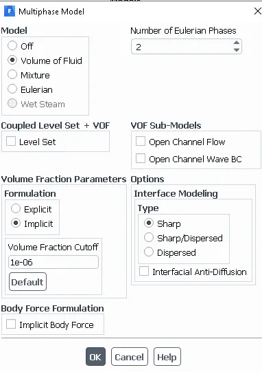
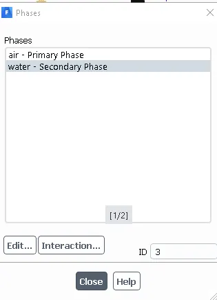
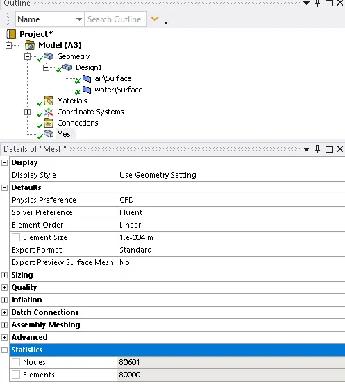
Setup and Solution:
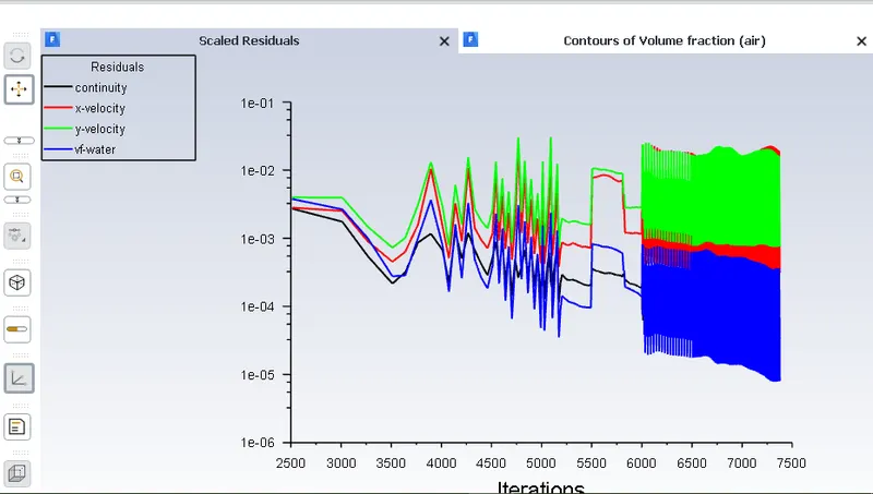
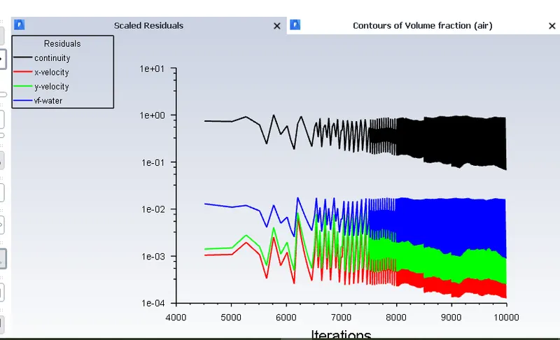
Residual Plot:
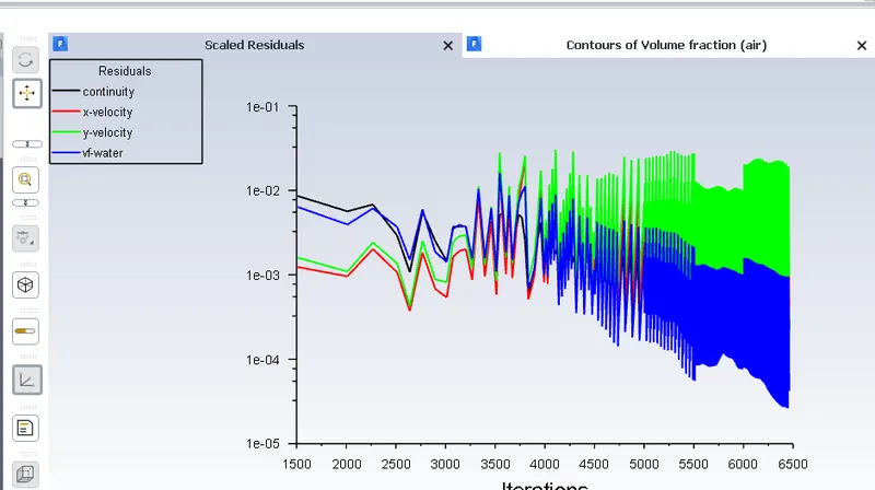
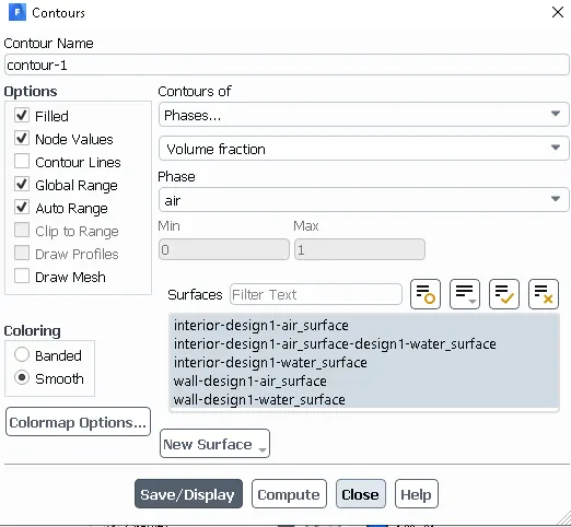
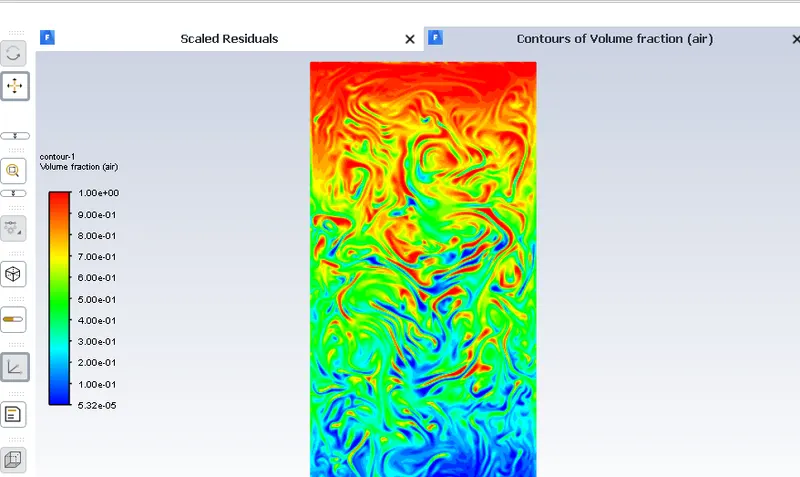
Contour Plot:
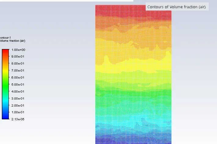
Animation Link:
4. Define the Atwood Number. Find out the Atwood number for both the cases and explain how the variation in Atwood number in the above two cases affects the behavior of the instability.
The Atwood number (A) is a dimensionless number in fluid dynamics used in the study of hydrodynamic instabilities in density stratified flows. It is a dimensionless density ratio defined as

where
 = density of heavier fluid
 = density of lighter fluid