Week 3 - Solving second order ODEs

Aim: To write a program in Matlab that will Simulate the pendulum motion,just like the one shown in the start of this challenge.

Gorverning Equation and Diagram:

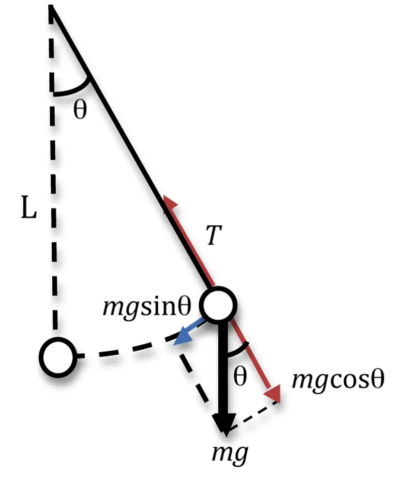
Second order differetial equation of simple pendulum:

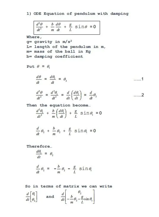
t = 0 to 20

b = 0.05

m = 1

L = 1

g = 9.81

Objective of the program:

To study the 2nd order differential equation in matlab for that we consider simple motion of pendulum.

Body of the content:

clear all
close all
clc

b = 0.05;
g = 9.81;
l = 1;
m = 0.1;

% intial condition
theta_0 = [0;3];

% time points
t_span = linspace(0,20,500);

% solve ODE
[t,results] = ode45(@(t,theta) ode_func(t,theta,b,g,l,m),t_span,theta_0);
figure(1)
plot(t,results(:,1))
hold on
plot(t,results(:,2))
ylabel('angular velocity')
xlabel('time')

figure(2)
ct = 1;
for i = 1:length(results(:,1))
    a = (results(i,1));
    
    x_start = 0;
    y_start = 0;
    
    x_end = l*sin(a);
    y_end = -l*cos(a);
    
    % plot
    plot([-1 1],[0 0],'linewidth',2,'color','r') % ceiling line
    hold on
    plot([x_start x_end],[y_start y_end],'color','black','linewidth',1) % string length
    plot(x_end,y_end,'o','markersize',20,'markerfacecolor','y') % mass of the ball
   
    grid
    axis([-1.5 1.5 -1.5 1])
    pause(0.03)
    M(ct) = getframe(gcf);
    ct = ct+1;
end

movie(M)
videofile = VideoWriter('simple_pendulum.avi','Uncompressed AVI');
open(videofile)
writeVideo(videofile,M)
close(videofile)

function [dtheta_dt] = ode_func(t,theta,b,g,l,m)

theta1 = theta(1)
theta2 = theta(2)
dtheta1_dt = theta2;
dtheta2_dt = -(b/m)*theta2-(g/l)*sin(theta1);
dtheta_dt = [dtheta1_dt; dtheta2_dt];
end

Explanation of the program:

1. First step implement intial values for t,theta,b,g,l,m.

2. After that define the time span as 0 to 20 secs and divided into 500 equal interval using linspace command.

3. To solve the second order differential use ode45 command.

4. After that create a separate function file in that we create a function i:e ode_func(t,theta,b,g,l,m) and save the program with the same function name.

5. After that run the ode_func(t,theta,b,g,l,m) in command window after that output of first program will display.

6. Then plot(t,results(:,1))

7. Use hold on command.

8. Then again plot(t,results(;,2))

9. After that label the plot xlabel(time) and ylabel(angular velocity)

10. Next step is to create simple pendulum motion in animation for that animation we use for loop coomand.

11. First fix the point of pendulum i:e x_start and y_start.

12. Then give inputs to another end of pendulum i:e x_end and y_end.

13. After that plot the co-ordinates i:e [-1 1] and [0 0] for ceiling line.

14. Then use hold on command.

15. Plot the string of the pendulum i:e [x_start x_end] and [y_start y_end].

16. lastly plot ball of the pendulum at x_end and y_end.

17. To create sphere use markersize command and for sphere color use markerfacecolor command.

18. use grid on command.

19. Then mention axis and use pause.

20. M(ct) = getframe(gcf) command for animation.

21. lastly use movie(M) coomand to create videofile.

22. saved videofile use videofile = VideoWrite('simple_pendulum.avi','uncompressed AVI')

23. Then close videofile and enter f5 output will be generated.

Errors:

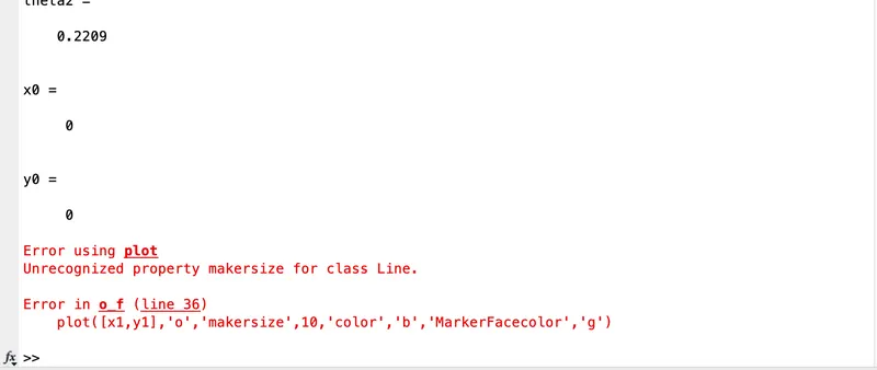
spelling mistake in markersize command

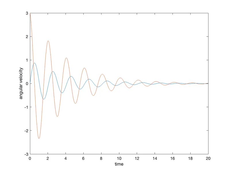
Results: Plot time vs angular velocity:

Animation link:

https://youtu.be/5xeqVfOVtAQ

Conclusion:

1. The graph time vs angular velocity is plotted.

2. Animation of simple pendulum is created.