Project 2 - Rankine cycle Simulator

Aim: Craete a Rankine Cycle Simulator using Matlab.

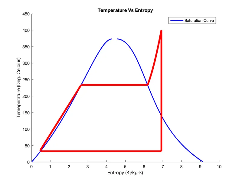
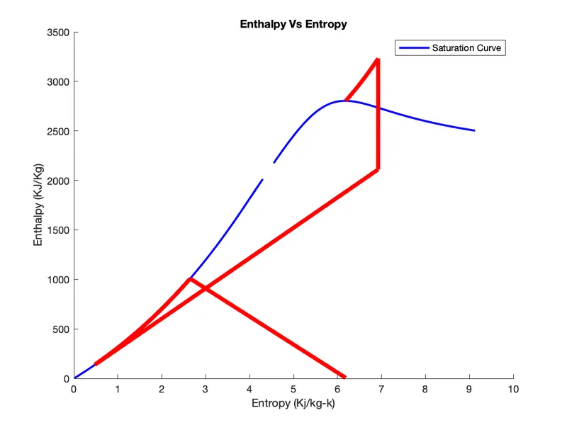
1. Plot the corresponding T-s and h-s plots for the given sets of inputs.Title and axes labels are a must,While legends could be used if necessary.

2. Attach the Report expalining the working of a Rankine Cycle Simulator.

Detail Explanation of Rankine Cycle Simulator and all equations required for this Cycle:

1. What is Rankine Cycle?

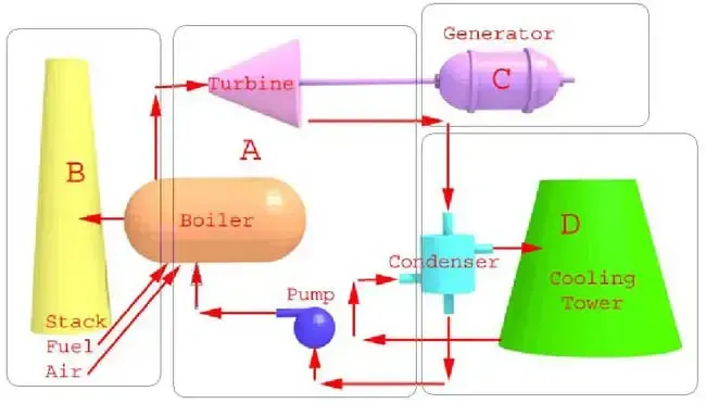
The Rankine cycle or Rankine Vapor Cycle is the process widely used by power plants such as coal-fired power plant or nuclear reactors. In this mechanism, a fuel is used to produce heat within a boiler, converting water into steam which then expands through a turbine producing useful work. This process was developed in 1859 by Scottish engineer William J.M. Rankine.This is a thermodynamic cycle which converts heat into mechanical energy—which usually gets transformed into electricity by electrical generation.

The four processes in the Rankine Cycle:

There are four processes in the Rankine cycle.

• Process 1–2: The working fluid is pumped from low to high pressure. As the fluid is a liquid at this stage, the pump requires little input energy. Process 1-2 is isentropic compression.
• Process 2–3: The high-pressure liquid enters a boiler, where it is heated at constant pressure by an external heat source to become a dry saturated vapour. The input energy required can be easily calculated graphically, using an enthalpy-entropy chart, or numerically, using steam table or software. Process 2-3 is constant pressure heat addition in boiler.
• Process 3–4: The dry saturated vapour expands through a turbine, generating power. This decreases the temperature and pressure of the vapour, and some condensation may occur. The output in this process can be easily calculated using the chart or tables noted above. Process 3-4 is isentropic expansion.
• Process 4–1: The wet vapour then enters a condenser, where it is condensed at a constant pressure to become a saturated liquid. Process 4-1 is constant pressure heat rejection in condenser.

Variables:

	Heat flow rate to or from the system (energy per unit time)
	Mass flow rate (mass per unit time)
	Mechanical power consumed by or provided to the system (energy per unit time)
	Thermodynamic efficiency of the process (net power output per heat input, dimensionless)
	Isentropic efficiency of the compression (feed pump) and expansion (turbine) processes, dimensionless
	The "specific enthalpies" at indicated points on the T-s diagram.
	The final "specific enthalpy" of the fluid if the turbine were isentropic.
	The pressures before and after the compression process.

Governing Equation:

1.Workdone for turbine in the rankine cycle

W_T = h1-h2

2.Workdone for pump

3.W_P = v3*(p4-p3)*100

h4 = W_P+h3

4.Net workdone in a Rankine Cycle

W_net = W_T-W_P

5.Heat aadition to system

Q1 = h1-h4

6.heat rejection to system

Q2 = h2-h3

7.Thermal Efficiency of Rankine Cycle

T_E = (W_net/Q1)*100

8.Specific Steam Consumption

S_S_C = 3600/W_net

9.Back work ratio

B_W_R = W_P/W_T

inputs

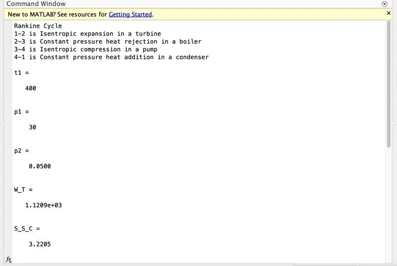
t1 = 400

p1 = 30

p2 = 0.05

Difference between Ideal and Actual Rankine Cycle:

The efficiency of the ideal Rankine cycle is close to the efficiency of the Carnot Cycle.

But in real plants, each stage of the Rankine cycle is associated with some irreversible processes. Thus the efficiency of the actual Rankine cycle is far lower than the ideal Rankine cycle efficiency.

Given below Fig. 1-a and Fig 1-b represents the Rankine cycle on P-v and T-s diagram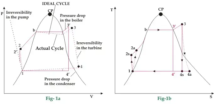

Rankine Cycle Representation is as follows on P-v and T-s diagrams:
Ideal Rankine Cycle	1-2‘-b-3‘-4‘-1
Actual Rankine Cycle	1-2-b-3-4-1

Critical Point (CP) is in the curve’s center, as shown in Fig 1-a and 1-b above. The curved lines on the left side of the CP are saturated-liquid lines, and the region/area to the left of these lines are called sub-cooled liquid regions.

Similarly, curved lines on the right side of the CP are saturated- vapor lines and the region/area to the right of these lines are called super-heat vapor regions.

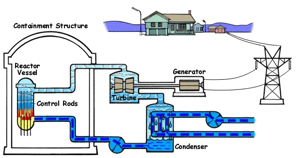
Working of Rankine Cycle in nuclear power plant:

Body of the Content:

Write code in Matlab for Rankine Cycle Simulator:

clear all
close all
clc

disp('Rankine Cycle');
disp('1-2 is Isentropic expansion in a turbine');
disp('2-3 is Constant pressure heat rejection in a boiler');
disp('3-4 is Isentropic compression in a pump');
disp('4-1 is Constant pressure heat addition in a condenser');

% inputs 
 t1 = 400   % Turbine inlet temperature in degree celcius
 p1 = 30     % Turbine inlet pressure in bar
 p2 = 0.05   % Condenser inlet pressure in bar
 
 % Obtaining data from Xsteam file for state 1
 %Enthalpy
 h1 = XSteam('h_pT',p1,t1);
 % Entropy
 s1 = XSteam('s_pT',p1,t1);
 
 % State 2
 s2 = s1;
 sf2 = XSteam('sL_p',p2);
 sg2 = XSteam('sV_P',p2);
 x2 = (s2-sf2)/(sg2-sf2);
 hf2 = XSteam('hL_p',p2);
 hg2 = XSteam('hV_p',p2);
 h2 = hf2+(x2*(hg2-hf2));
 
 % state 3
 p3 = p2;
 s3 = XSteam('sL_p',p3);
 h3 = XSteam('hL_p',p3);
 
 % state 4
 s4 = s3;
 p4 = p1;
 
 % Workdone for turbine in the rankine cycle
 W_T = h1-h2
 
 % Workdone for pump
v3 = XSteam('vL_p',p3);
W_P = v3*(p4-p3)*100;
h4 = W_P+h3;

% Net workdone in a Rankine Cycle
W_net = W_T-W_P;

% Heat aadition to system
Q1 = h1-h4;

% heat rejection to system
Q2 = h2-h3;

% Thermal Efficiency of Rankine Cycle
T_E = (W_net/Q1)*100;

% Specific Steam Consumption 
S_S_C = 3600/W_net

% Back work ratio
B_W_R = W_P/W_T
 
% Temperature and other constant
t3 = XSteam('Tsat_p',p3);
t2 = t3;
Cp4 = XSteam('Cp_ps',p4,s4);
Cv4 = XSteam('Cv_ps',p4,s4);
k = Cp4/Cv4
t4 = t3/((p3/p4)^((k-1)/k));
t6 = XSteam('Tsat_p',p1);
s5 = XSteam('sL_p',p1);
s6 = XSteam('sV_p',p1);
h5 = XSteam('hL_p',p1);
h6 = XSteam('sV_p',p1);
t5 = t6;

%Plotting for Saturation Line
T = linspace(1,500,1000);
for i = 1:length(T)
    sf(i) = XSteam('sL_T' ,T(i));   % Saturated Liquid Entropy
    sg(i) = XSteam('sV_T' ,T(i));   % Saturated Vapour Entropy
    hf(i) = XSteam('hL_T' ,T(i));   % Saturated Liquid Enthalpy
    hg(i) = XSteam('hV_T' ,T(i));   % Saturated Vapour Enthalpy
    
end

% Plotting T-S Diagram for Rankine Cycle
figure(1)
hold on
plot(sf,T,'color','b','linewidth',2)
plot(sg,T,'color','b','linewidth',2)
plot([s1 s2],[t1 t2],'color','r','linewidth',4)
plot([s2 s3],[t2 t3],'color','r','linewidth',4)
plot([s3 s4],[t3 t4],'color','r','linewidth',4)
plot([s4 s5],[t4 t5],'color','r','linewidth',4)
plot([s5 s6],[t5 t6],'color','r','linewidth',4)
s_1 = linspace(s6,s1,1000);
for j = 1:length(s_1)
    Tc(j) = XSteam('T_ps',p1,s_1(j));
end
plot(s_1,Tc,'color','r','linewidth',4)
title('Temperature Vs Entropy')
xlabel('Entropy (Kj/kg-k)')
ylabel('Temeperature (Deg. Celcius)')
legend('Saturation Curve')

% Plotting H-S Diagram for Rankine Cycle
figure(2)
hold on
plot(sf,hf,'color','b','linewidth',2)
plot(sg,hg,'color','b','linewidth',2)
plot([s1 s2],[h1 h2],'color','r','linewidth',4)
plot([s2 s3],[h2 h3],'color','r','linewidth',4)
plot([s3 s4],[h3 h4],'color','r','linewidth',4)
hc = linspace(h4,h5,100);
for k = 1:length(hc)
    s_c(k) = XSteam('s_ph',p1,hc(k));
end
plot(s_c,hc,'color','r','linewidth',4)
plot([s5 s6],[h5 h6],'color','r','linewidth',4)
for l = 1:length(s_1)
    h_c(l) = XSteam('h_ps',p1,s_1(l));
end
plot(s_1,h_c,'color','r','linewidth',4)
title('Enthalpy Vs Entropy')
xlabel('Entropy (Kj/kg-k)')
ylabel('Enthalpy (KJ/Kg)')
legend('Saturation Curve')

% Displaying Results in Command window

fprintf('At state point 1\t\t\t\t\t')
fprintf('At state Point 2\n')
fprintf('p1 = %10f in Bar\t\t\t\t',p1);
fprintf('p2 = %10f in Bar\n',p2);
fprintf('t1 = %10f in Deg.Celcius\t\t',t1);
fprintf('t2 = %10f in Deg.Celcius\n',t2);
fprintf('H1 = %10f in KJ/Kg\t\t\t',h1);
fprintf('H2 = %10f in KJ/Kg\n',h2);
fprintf('S1 = %10f in KJ/Kg-k\t\t\t',s1);
fprintf('S2 = %10f in KJ/Kg-k\n',s2);
fprintf('\n')
fprintf('At state point 3\t\t\t\t\t')
fprintf('At state Point 4\n')
fprintf('p3 = %10f in Bar\t\t\t\t',p3);
fprintf('p4 = %10f in Bar\n',p4);
fprintf('t3 = %10f in Deg.Celcius\t\t',t3);
fprintf('t4 = %10f in Deg.Celcius\n',t4);
fprintf('H3 = %10f in KJ/Kg\t\t\t',h3);
fprintf('H4 = %10f in KJ/Kg\n',h4);
fprintf('S3 = %10f in KJ/Kg-k\t\t\t',s3);
fprintf('S4 = %10f in KJ/Kg-k\n',s4);
fprintf('\n')
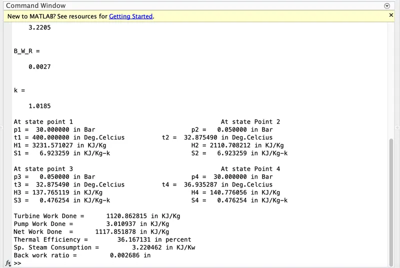
fprintf('Turbine Work Done = %16f in KJ/Kg\n',W_T)
fprintf('Pump Work Done = %16f in KJ/Kg\n',W_P)
fprintf('Net Work Done  = %16f in KJ/Kg\n',W_net)
fprintf('Thermal Efficiency = %16f in percent\n',T_E)
fprintf('Sp. Steam Consumption = %16f in KJ/Kw\n',S_S_C)
fprintf('Back work ratio = %16f in \n',B_W_R)

Explanation of code:

1. First is to download XSteam file and save in current directory.

2. First step of our coding is to display Rankine Cycle all four processes for that use disp command.

3. After that define the inputs which are provided

4. i) Obtaining data from XSteam file for stage 1 for enthalpy and entropy.

ii) Obtaining data from XSteam file for stage 2 for enthalpy and entropy.

ii) Obtaining data from XSteam file for stage 3 for enthalpy and entropy.

ii) Obtaining data from XSteam file for stage 4 for enthalpy and entropy.

5. After that define t3 and t4 temperature using XSteam file.

6. Define h5,h6,s5 and s6 through XSteam file.

7. Then calculate workdone for turbine in the cycle and same for pump.

8. Calculate heat addition and heat rejection in the system.

9. After that calculate Thermal Efficiency,Specifc steam consumption and Back work ratio.

10. Then plot T- s diagram and saturation line use linspace command and for loop command.

11. Mention the title,label and lastly use legend.

12. Then plot h- s diagram for that use linspace command and for loop command.

13. Lastly use fprintf command to display all the results command window.

Results: Outputs

Plots: 1.Temperature vs entropy

Plot: 2.Enthalpy vs Entropy

References:

https://www.electrical4u.com/ideal-verses-actual-in-rankine-cycle/

https://en.wikipedia.org/wiki/Rankine_cycle

https://energyeducation.ca/encyclopedia/Rankine_cycle

Conclusion:

1. We sucessfully create a Rankine Cycle Simulator using Matlab

2. Also we sucessfully plot the T-s and h-s.