Week 5 - Rayleigh Taylor Instability
Rayleigh Taylor Instability:
RT instability (after Lord Rayleigh and G. I. Taylor) is the instability of the interface between two immiscible fluids of different densities which occurs when lighter fluid is pushing the heavier fluid.
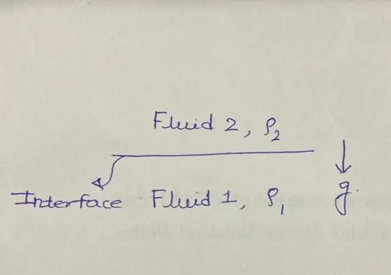
if `rho_1>rho_2` then it is a stable configuration
if `rho_2>rho_1` then it is an unstable configuration
if somehow I put a heavier fluid over the lighter, then lighter fluid will go up and heavier fluid will go down. hence overturning will take place. this is called as Rayleigh Taylor Instability.
Assumptions:
- fluids have zero viscosity (inviscid)
- fluids are unbounded (means fluid 1,2 go infinity in vertical upward and downward direction respectively)
Physical variables:
| Variables | Dimension |
| Fluid density, `rho_1` | `ML^-3` |
| Fluid density, `rho_2` | `ML^-3` |
| Interfacial tension, `gamma` | `MT^-2` |
| Acceleration due to gravity, g | `LT^-2` |
The above table shows that there are three fundamental dimensions (`M, L, T`) and four variables. so by using Buckingham `pi`, we get a Non-dimensional number that is called Atwood Number.
Atwood Number (`A_t`):
It is defined as the ratio of density difference to total density.
`A_t=(rho_1-rho_2)/(rho_1+rho_2)`
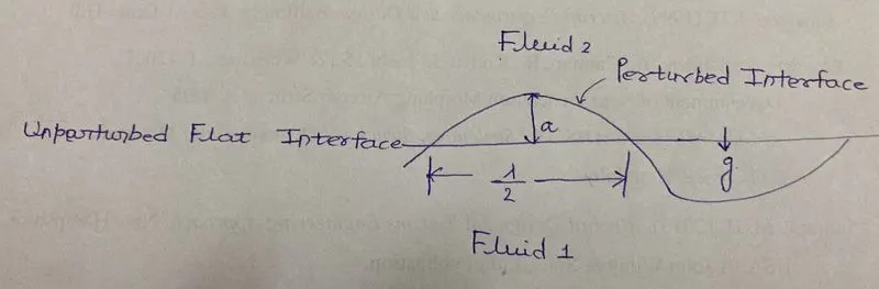
Here,
`lambda`=Wavelength
`k=(2pi)/lambda`=Wave number
The volume of fluid per unit width `prop` `atimes(lambda/2)`
the volume of fluid per unit width `prop a/k`
Net bouncy force per unit width `prop a/k(rho_2-rho_1)g`
`ifrho_2>rho_1`then it is called as destable force.
`if rho_1>rho_2`then it is called as stable force. means bouncy force will act in downward direction.
practical CFD models based on the mathematical analysis of Rayleigh Taylor waves:
- Richtmyer-Meshkov instability: occurs when two fluids of different density are impulsively accelerated. Normally this is by the passage of a shock wave. The development of the instability begins with small amplitude perturbations which initially grow linearly with time. This is followed by a nonlinear regime with bubbles appearing in the case of a light fluid penetrating a heavy fluid, and with spikes appearing in the case of a heavy fluid penetrating a light fluid. A chaotic regime eventually is reached and the two fluids mix. This instability can be considered the impulsive-acceleration limit of the Rayleigh-Taylor instability.
- Kelvin–Helmholtz instability: it is a fluid instability that occurs when there is velocity shear in a single continous fluid or a velocity difference across the interface between two fluids. example: cloud formation on earth

- Plateau–Rayleigh instability: often just called the Rayleigh instability, explains why and how a falling stream of fluid breaks up into smaller packets with the same volume but less surface area. It is related to the Rayleigh-Taylor instability and is part of a greater branch of fluid dynamics concerned with fluid thread breakup. This fluid instability is exploited in the design of a particular type of ink jet technology whereby a jet of liquid is perturbed into a steady stream of droplets.

Q.1 Perform the Rayleigh Taylor instability simulation for 2 different mesh sizes with the base mesh being 0.5 mm. Compare the results by showing the animations( Attach them from your google drive). Observe the differences in the animation and explain the effect of mesh size on simulation. Also, explain why a steady-state approach might not be suitable for these types of simulation.[ Choose Air and Water for this simulation]
Following steps, we are going to do.
- Geometry
- Mesh
- Setup
- Solution
- Result
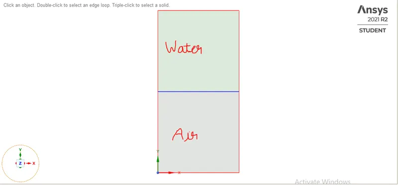
1. Geometry:
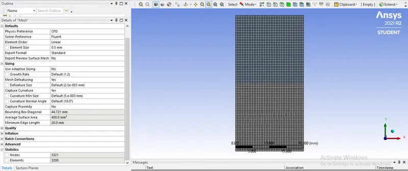
2. Mesh (size=0.5 mm):
3. Setup:
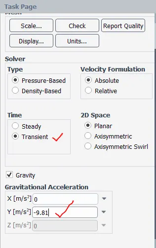
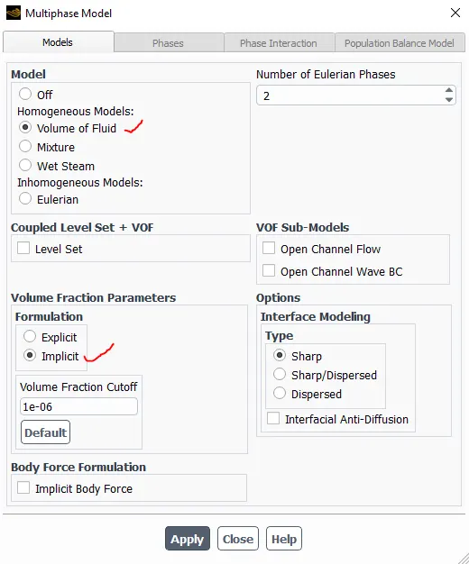
Now we enabal the multiphase model. under the multiphysics model we choose " Volume of Fluid" model. because in VOF, we are going to find out the position of interface between air and water. hence in this VOF, volume fraction of each fluid in each cell can be tracked. in the given domain we have two phases. one is air that is in gas phase and above it we have water that is in liquid phase. that is why we are putting 2 in "Number of Eulerian Phases".
Volume fraction represents the space occupied by water and air in a cell. that is 1e-6. Volume fraction is denoted by `alpha`
`alpha_a+alpha_w=1`
Here, `alpha_a` is the volume faction of air
`alpha_w`is tha volume fraction of water
Volume of fraction equation for water(`alpha_w`):
`1/rho_w[(del)/(delt)(alpha_wrho_w)+grad.(alpha_wrho_wv_w)=S_(alpha_w)+dotm_(aw)-dotm_(wa)]`
now we can solve the above equation either implicit or explicit. so here we are choosing implicit option.
`(alpha_w^(n+1)rho_w^(n+1)-alpha_w^nrho_w^n)/(Deltat)+sum(rho_w^(n+1)U_f^(n+1)alpha_(w,f)^(n+1))=sum[S_(alphaw)+dotm_(wa)-dotm_(aw)]V`
Volume of fraction for air=1-Volume of fraction for water
`alpha_a=1-alpha_w`
by using above two red colour equations, analytically we find the volume fraction of water `alpha_w` and air `alpha_a`. alongwith paralley we are also finding out `alpha_w and alpha_a` by doing simulation.
Multiphase Model Selection:
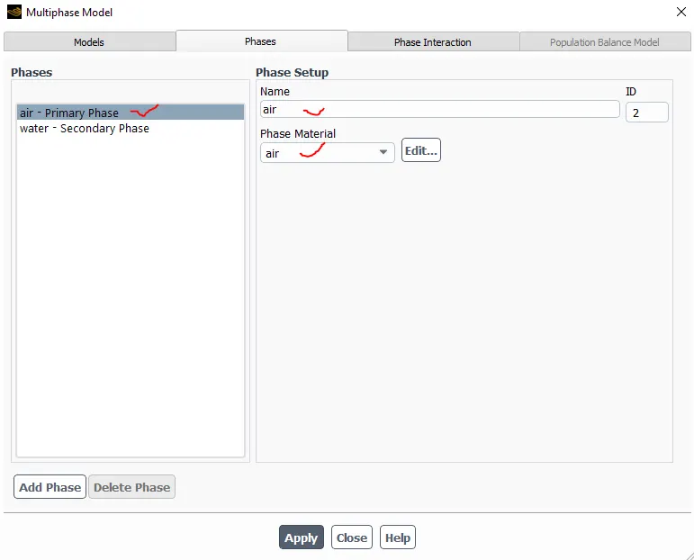
Phase selection:
Primary phase-air
Secondary phase-water
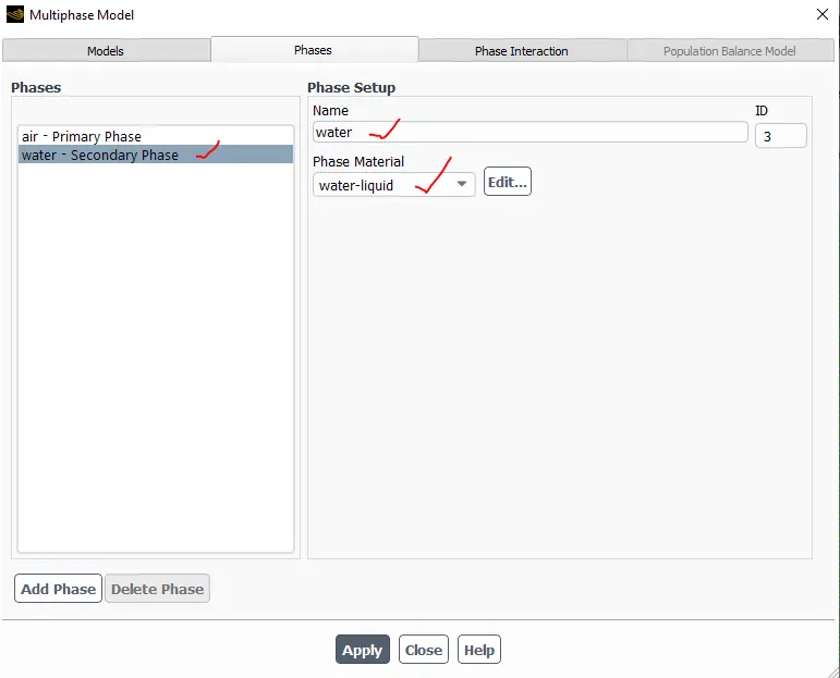
Material Selection:
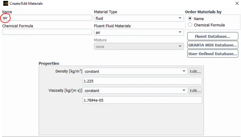
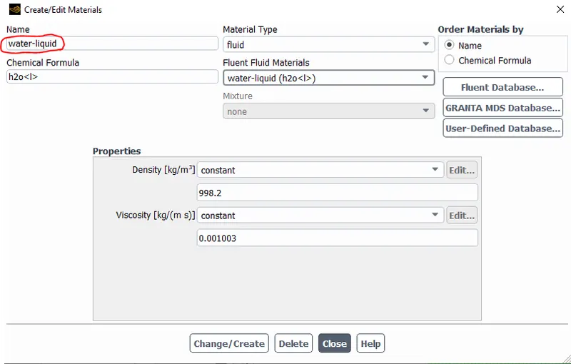
`A_t=(rho_1-rho_2)/(rho_2+rho_2)=(998.2-1.225)/(998.2+1.225)=0.99754`
Patch:
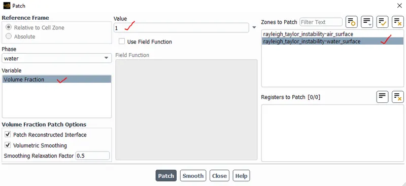
In above figure, volume fracion of water `alpha_w=1`
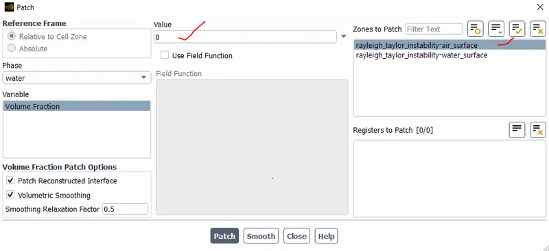
In the above figure, volume fraction of air `alpha_a=0`
Hence total volume=1
`alpha_w+alpha_a=1`
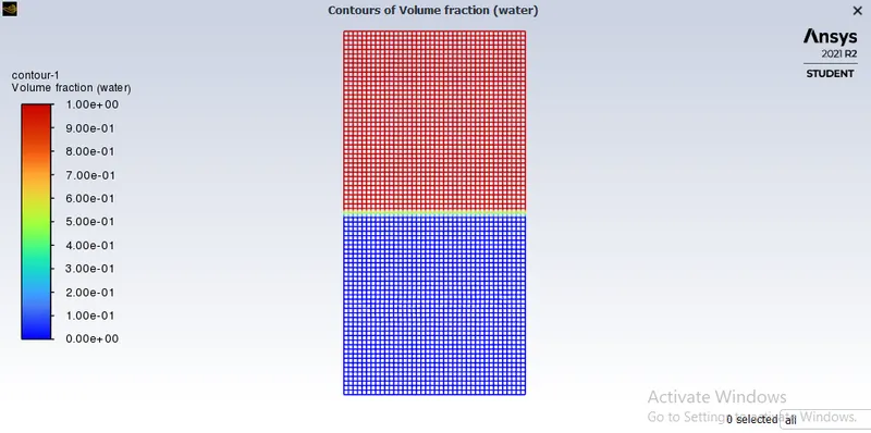
the above figure gives the confirmation that the volume fraction of water is 1 (red colour) and the volume fraction of air is 0 (blue colour).
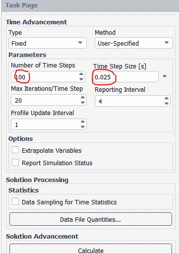
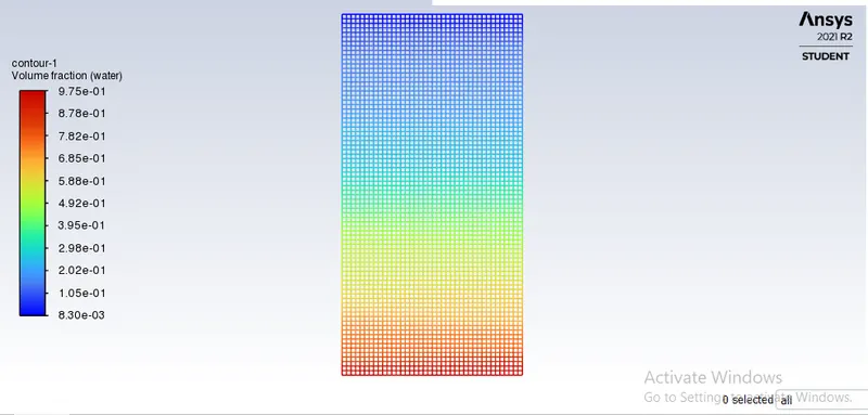
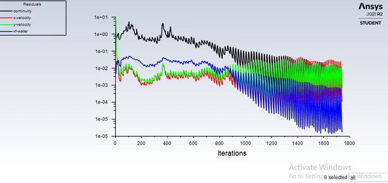
5. CFD Post:
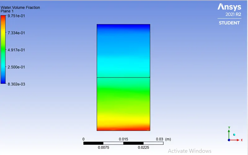
Google drive link of the volume of a fraction of water (baseline simulation of size 0.5 mm):
https://drive.google.com/file/d/1NDozkKFOai_aq3UbXasiq2ewzNDk18b5/view?usp=sharing
Case 2: Mesh (element size=0.25 mm)
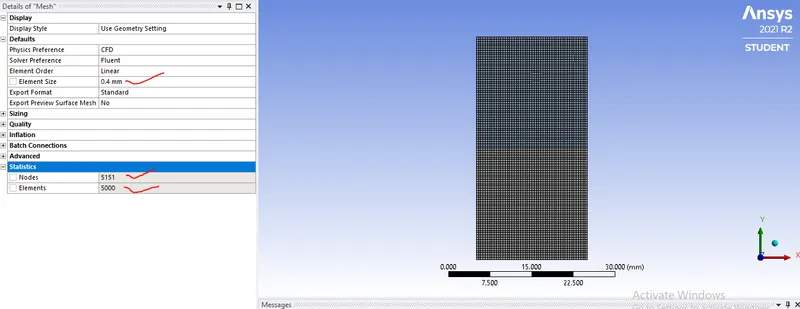
3.Setup:
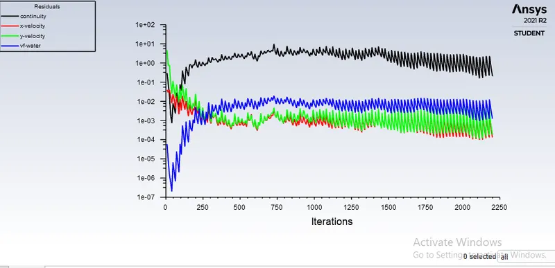
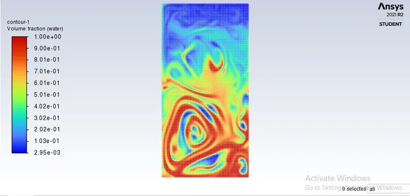
google drive link of Volume fraction of refined mesh(0.25 mm)
https://drive.google.com/file/d/1zksx1mxmJwxe9EglXCVfzQcaArzrMWS3/view?usp=sharing
5. CFD Post:
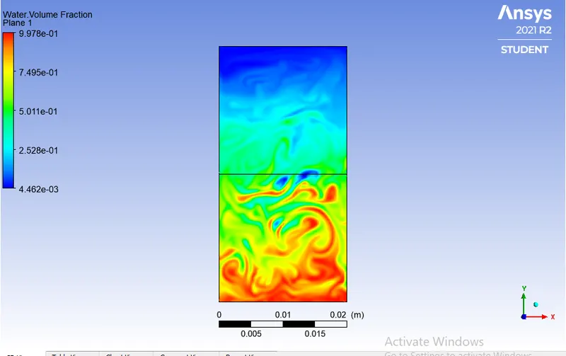
Case 3: Transient (Water + User defined material) 0.5 mm mesh size
- density=400 kg/m3
- viscosity= 0.001 kg/m-s
Why Steady state simulation doesnot suitable for Rayleigh Taylor Instability simulation ?
- steady state means that flow variable does not change with time at particular location. hence it will not capture any variation in simulation.
- as we know that, time derivative terms are involved in below governing equation. but due to steady state, solver ignores that time derivative terms.
- `(alpha_w^(n+1)rho_w^(n+1)-alpha_w^nrho_w^n)/(Deltat)+sum(rho_w^(n+1)U_f^(n+1)alpha_(w,f)^(n+1))=sum[S_(alphaw)+dotm_(wa)-dotm_(aw)]V`