Week 5 - Rayleigh Taylor Instability

AIM

Perform the Rayleigh Taylor instability simulation for 2 different mesh sizes with the base mesh being 0.5 mm. Compare the results by showing the animations( Attach them from your google drive). Observe the differences in the animation and explain the effect of mesh size on simulation. Also, explain why a steady-state approach might not be suitable for these types of simulation.[ Choose Air and Water for this simulation]

OBJECTIVES

1. What are some practical CFD models that have been based on the mathematical analysis of Rayleigh Taylor waves? In your own words, explain how these mathematical models have been adapted for CFD calculations.
3. Run one more simulation with water and user-defined material(density = 400 kg/m³, viscosity = 0.001 kg/m-s) for refined mesh.
4. Define the Atwood Number. Find out the Atwood number for both the cases and explain how the variation in Atwood number in the above two cases affects the behavior of the instability.

RT instabiliy is used in many areas, the models are listed below

1. saffman -Taylors instability (viscosity fingering ) this instability created when there is no exteernal force for the displacement is provided. the less viscous fluid injected in the high viscouus fluid it further pushes the highly viscous fluid in down stream to create fingering effect
2. richetmyer- Meshkov instability used when a external agent is required for accelarating the flow this instability we obsereve when we imuplssively accelarate the different viscous and density fluids. penetratio of lighter fluid into heavy fluid happens and spikes observe in the highly viscous fluid, after a chaotic regime the both fluids get mixed. EX. scramjet engine
3. Platue_rayleigh instability similer to rayleigh taylor instabilty. focuses on fluid thread break up as a part of fluid dynamics( the one part of fluid flow break into several small bubble because of the surface tension and area of contact). examples are inkjet flow. inkjet printers and water dripping.

Modeling approach

case 1 mesh size is 0.5 mm (base mesh)

case 2 mesh size is 0.25mm (refined mesh)

case 3 simulation with user defined material with denity 400 kg/m^3 and viscosity 0.001 kg/m-s with mesh size 0.25mm

PROCEDURE

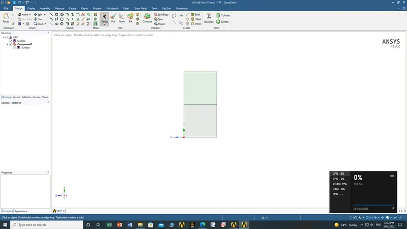
1 GEOMETRY

2.MESHING

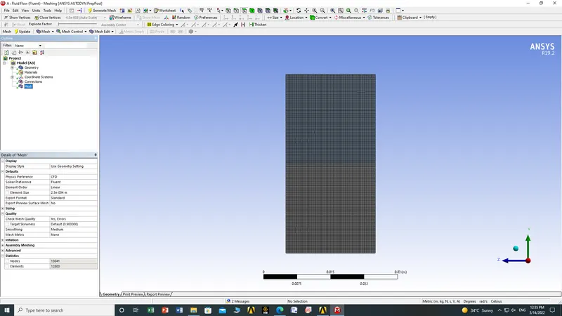
BASE MESH (0.0005 m)

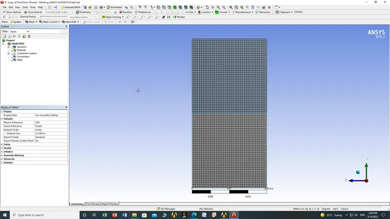
(REFINED MESH 0.00025 m )

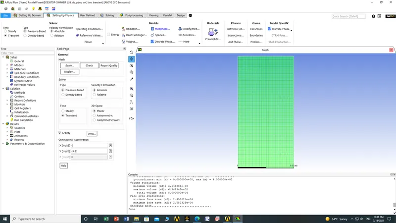
FLUENT SET UP

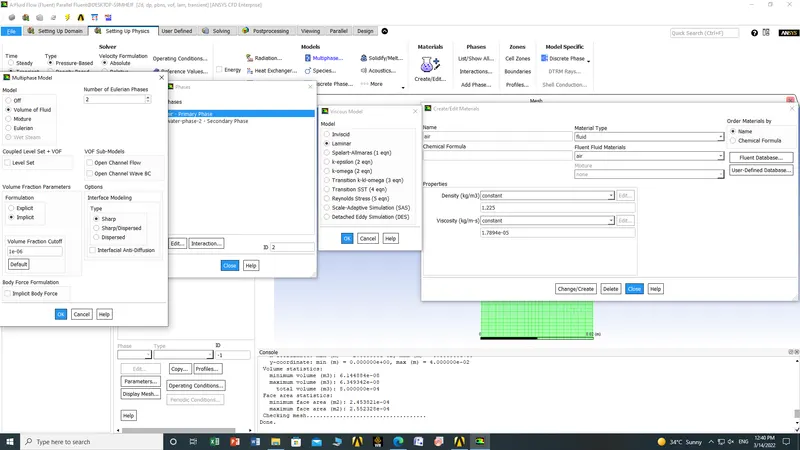
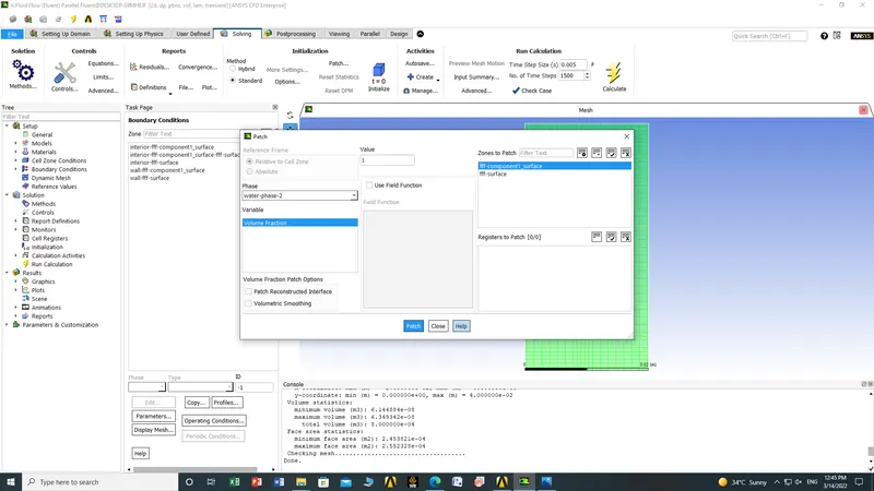
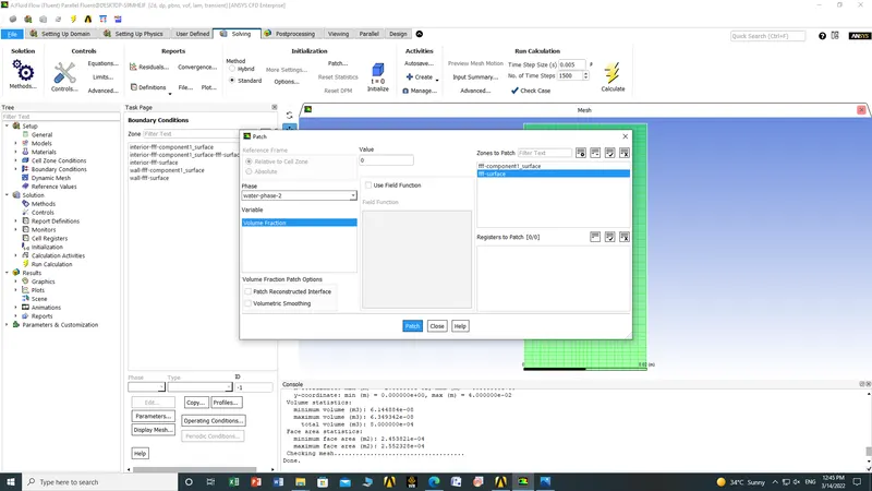
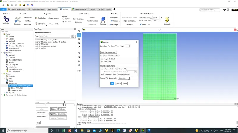
RESULTS FOR BASE MESH

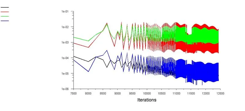
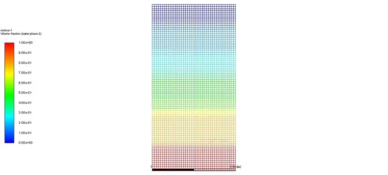
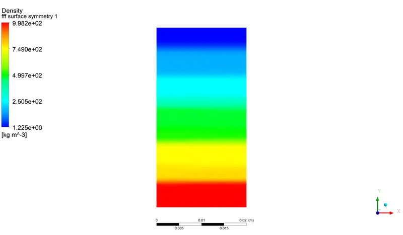
https://drive.google.com/file/d/1fjc7DGKtb6X1sZYnhSmwxIeXayVVKcjH/view?usp=sharing

RESULTS (FOR REFINED MESH)

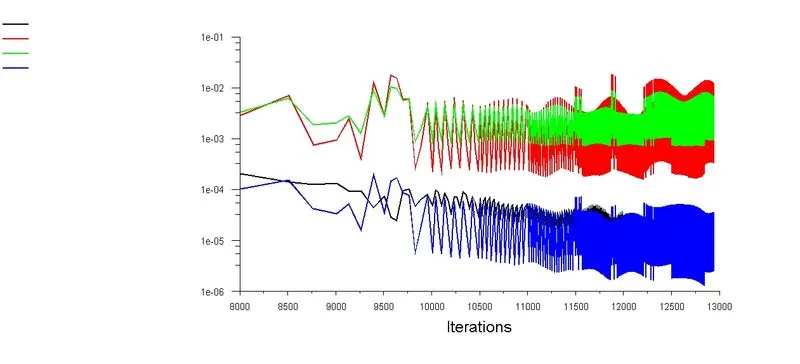
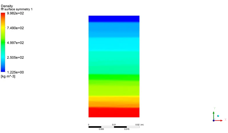
https://drive.google.com/file/d/1ppJH5LBQHyp_64w6dJQr7M3Z9TWtA_g-/view?usp=sharing

CASE 3 SIMULATING WITH WATER AND USER DEFINED MATERIAL (density = 400 kg/m³, viscosity = 0.001 kg/m-s)

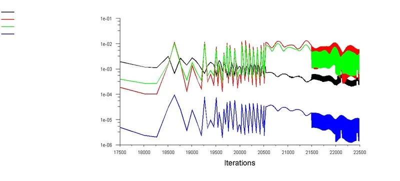
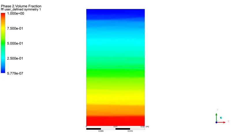
https://drive.google.com/file/d/1rc_vJaPwe81nv8pXayZJ4O85BVW99hfa/view?usp=sharing

ATWOOD NUMBER a non dimenssional number used to examine the study of hydrodyanmic instabilities in density strafucation flows

it us the ratio os density difference of two phases to the density sum of different flows

for case 1 and 2 atwood number is 0.9975

for case e atwood number is 0.427

CONCLUSSIONS

1. incase of innstability volume fractions are functions of time
2. as the atwwod number increses mixing effects will be lowererd
3. as the mesh become finer we can capture flow effectivey and effcets the convergence of hydrodynamic instability