Project 2 - Rankine cycle Simulator
Aim: To create a Rankine cycle simulator simulator
objective
1. to draw saturation curve
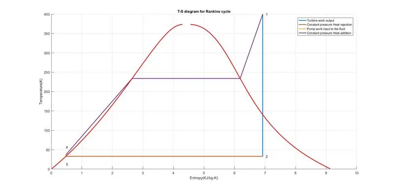
2. to draw T-S plot of Rankine cycle
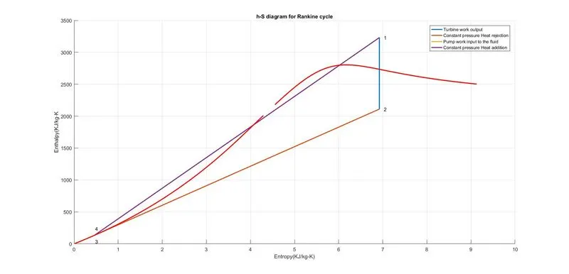
3. to draw an H-S plot of the Rankine cycle
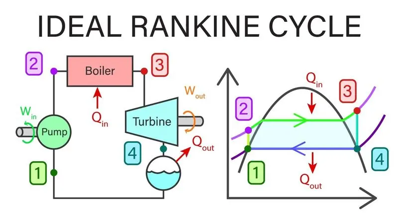
Rankine cycle is the ideal cycle for steam power plants
following are the different process in Rankine cycle
1-2 Isentropic expansion in the turbine
2-3 constant pressure heat rejection
3-4 isentropic compression
4-1 constant pressure heat addition
turbine work =h1-h2;
pump work= v3(p4-p3);
heat addition= h1-h4;
heat rejection=h2-h3;
line diagram of simple Rankine is shown below
the main program and stepwise explanation coding is shown below
%% write a code for rankine cycle
clear all % clears all the temporary files
close all % closes all the plots
clc       % clear the command window
% defining the input parameters of the turbine
t1= 400; % temperature at state 1 in K
p1=30;   % pressure at state 1 in Bars
h1= XSteam('h_pT',p1,t1); % enthalpy at state 1 in in kj/kg-k
s1=XSteam('s_pT',p1,t1);  % entropy at state 1 in in kj/kg-k
% defining the out put parameters of turbine
p2=0.05;   % pressure at state 2 in Bars
s2=s1;       % entropy at state 2 in in kj/kg-k
sf3=XSteam('sL_p',p2);  % entropy at state 3 in in kj/kg-k
sg2=XSteam('sv_p',p2);  % entropy at saturated state in in kj/kg-k
x=(s1-sf3)/(sg2-sf3);   % condition of steam outlet from the turbine
hf3=XSteam('hl_p',p2);  % enthalpy at saturated vapour state in in kj/kg-k
hg2=XSteam('hV_p',p2);  % enthalpy at saturated liquid state in in kj/kg-k
h2=hf3+x*(hg2-hf3);      % enthalpy at state 2 in in kj/kg-k
% work out put of the turbine
WT=h1-h2;
% defining the inlet parameters to the pump
p3=p2;                   % pressure at state 3 in Bars
t3=XSteam('Tsat_p',p2);  % temperature at state 3 in K
t2 = t3;                 % temperature at state 2 in K
h3=hf3;                  % enthapy at state 3 in in kj/kg-k
s3=sf3;                  % entropy at state 3 in in kj/kg-k
vf3=XSteam('vl_p',p2);   % specific volume of the fluid at sate 3
% work done by the pump on fluid
WP=vf3*(p1-p3)*100;
% defining the outlet parameters of the pump
p4=p1;                   % pressure at state 4 in Bars
s4=s3;                   % entropy at state 3 in in kj/kg-k
h4=WP+h3;                %enthapy at state 4 in in kj/kg-k
cp4=XSteam('cp_ps',p4,s4); %specific heat atP=C at state 4
cv4=XSteam('cv_ps',p4,s4);  %specific heat atV=C at state 4
g4=cp4/cv4;                 %specific heat ratio
o=(g4-1)/g4;
t4=t3*(p4/p3)^o;             % temperature at state 4 in K

% defining the parameter at sate 5
t5=XSteam('Tsat_p',p1);       % temperature at state 5 in K
s5=XSteam('sl_p',p1);         % entropy at state 5 in in kj/kg-k
p5=p1;                        % pressure at state 5 in Bars
h5=XSteam('hl_p',p1);         %enthapy at state 5 in in kj/kg-k
%defining the parameters at state 6
t6=t5;                        % temperature at state 6 in K
s6=XSteam('sv_p',p1);         % entropy at state 6 in in kj/kg-k
p6=p1;                        % pressure at state 6 in Bars
h6=XSteam('hv_p',p1);          %enthapy at state 6 in in kj/kg-k
%performance parameters of rankine cycle
Wnet=WT-WP;                    %net work outpu of the turbine
BWR=WP/WT;                     % back work ratio
Qin=h1-h4;                     % heat input to rankkine cycle
eff= (WT-WP)/Qin;              %efficiency of the cycle
SSC=3600/WT;                   % pecific steam consumption of the cycle

%ploting saturation curve
T=linspace(1,700,1500);
for i=1:length(T)
    sf(i)=XSteam('sl_T',T(i));
    sg(i)=XSteam('sv_T',T(i));
    hf(i)=XSteam('hl_T',T(i));
    hg(i)=XSteam('hv_T',T(i));
end
figure(1)
hold on
%ploting temperature and entropy cuve for rankine cycle
plot([s1 s2],[t1 t2],'linewidth',2)
plot([s2 s3],[t2 t3],'linewidth',2)
plot([s3 s4],[t3 t4],'linewidth',2)
plot([s4 s5 s6 s1],[t4 t5 t6 t1],'linewidth',2)
plot(sf,T,'r','linewidth',2)
plot(sg,T,'r','linewidth',2)

% giving state point sti the rankine cycle
s=linspace(s6,s1,1500);
for j=1:length(s);
    T(j)=XSteam('T_ps',p1,s(j));
end

    text(s1+0.1, t1,'1');
    text(s2+0.1, t2,'2');
    text(s3,t3-20,'3');
    text(s4,t4+20,'4');
xlabel('Entropy(KJ/kg-K)')
ylabel('Temperature(K)')
title('T-S diagram for Rankine cycle')
grid on
legend('Turbine work output','Constant pressure Heat rejection','Pump work input to the fluid','Constant pressure Heat addition')
hold off
figure(2)
hold on
% ploting enthalpy and entropy plot of rankine cycle
plot([s1 s2 ],[h1 h2],'linewidth',2)
plot([s2 s3 ],[h2 h3],'linewidth',2)
plot([s3 s4 ],[h3 h4 ],'linewidth',2)
plot([s4 s1],[h4 h1],'linewidth',2)
plot(sf,hf,'r','linewidth',2)
plot(sg,hg,'r','linewidth',2)
%giving state points to hs plot of rankine cycle
sh=linspace(s6,s1,1500);
for k=1:length(sh);
    Th(j)=XSteam('T_ps',p1,s(k));
end

    text(s1+0.1, h1,'1');
    text(s2+0.1, h2,'2');
    text(s3,h3-100,'3');
    text(s4,t4+200,'4');
grid on
legend('Turbine work output','Constant pressure Heat rejection','Pump work input to the fluid','Constant pressure Heat addition')
xlabel('Entropy(KJ/kg-K)')
ylabel('Enthalpy(KJ/kg-K')
title('h-S diagram for Rankine cycle')
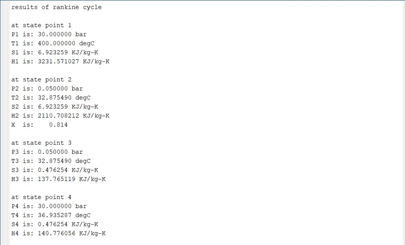
disp('results of rankine cycle')
fprintf('\n')
fprintf('at state point 1\n')
fprintf('P1 is: %f bar\n',p1)
fprintf('T1 is: %f degC\n',t1)
fprintf('S1 is: %f KJ/kg-K\n',s1)
fprintf('H1 is: %f KJ/kg-K\n',h1)
fprintf('\n')

fprintf('at state point 2\n')
fprintf('P2 is: %f bar\n',p2)
fprintf('T2 is: %f degC\n',t2)
fprintf('S2 is: %f KJ/kg-K\n',s2)
fprintf('H2 is: %f KJ/kg-K\n',h2)
fprintf('X  is: %8.3f\n',x)
fprintf('\n')
fprintf('at state point 3\n')
fprintf('P3 is: %f bar\n',p3)
fprintf('T3 is: %f degC\n',t3)
fprintf('S3 is: %f KJ/kg-K\n',s3)
fprintf('H3 is: %f KJ/kg-K\n',h3)
fprintf('\n')
fprintf('at state point 4\n')
fprintf('P4 is: %f bar\n',p4)
fprintf('T4 is: %f degC\n',t4)
fprintf('S4 is: %f KJ/kg-K\n',s4)
fprintf('H4 is: %f KJ/kg-K\n',h4)
fprintf('\n')
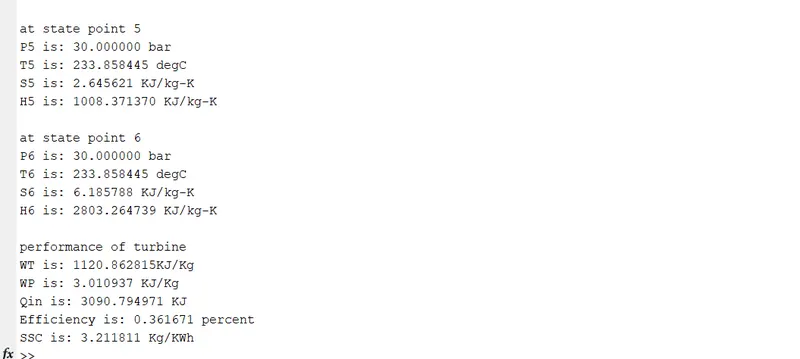
fprintf('at state point 5\n')
fprintf('P5 is: %f bar\n',p5)
fprintf('T5 is: %f degC\n',t5)
fprintf('S5 is: %f KJ/kg-K\n',s5)
fprintf('H5 is: %f KJ/kg-K\n',h5)
fprintf('\n')
fprintf('at state point 6\n')
fprintf('P6 is: %f bar\n',p6)
fprintf('T6 is: %f degC\n',t6)
fprintf('S6 is: %f KJ/kg-K\n',s6)
fprintf('H6 is: %f KJ/kg-K\n',h6)
fprintf('\n')
fprintf('performance of turbine\n')
fprintf('WT is: %fKJ/Kg\n',WT)
fprintf('WP is: %f KJ/Kg\n',WP)
fprintf('Qin is: %f KJ\n',Qin)
fprintf('Efficiency is: %f percent \n',eff)
fprintf('SSC is: %f Kg/KWh \n',SSC)
no errors have been found except typographical errors
Results and plots shown below