Week 3.5 - Deriving 4th order approximation of a 2nd order derivative using Taylor Table method
AIM
To derive the following 4th order approximations of the second-order derivative.
1. Central difference
2. Skewed right-sided difference
3. Skewed left-sided difference
OBJECTIVES
To prove that my skewed schemes are fourth-order accurate
To write a program in Matlab to evaluate the second-order derivative of the analytical function exp(x)*cos(x) and compare it with the 3 numerical approximations that you have derived.
To provide a plot that compares the absolute error between the above-mentioned schemes
In my own words, describe why a skewed scheme is useful? What can a skewed scheme do that a CD scheme cannot
CENTRAL DIFFERENCE SCHEME
NO.OF NODES =5;
(SINCE P+Q-1= NO.OF NODES, ORDER OF DERIVATIVE=P, Q IS THE ORDER OF APPROXIMATIONS)
=(af(i-2)+bf(i-1)+cf(i)+ df(i-1)+ ef(i-2))/dx2
(af(i-2)) = a ( f(i) - 2 f’(i)Δx/1! + 4 f’’(i)Δx2/2! - 8 f’’’(i)Δx3/3! + 16f’’’’(i)Δx4/4! - 32f’’’’’(i)Δx5/5! + -- - -)
(bf(i-1)) = b( f(i) - f’(i)Δx/1 + f’’(i)Δx2/2! - f’’’(i)Δx3/3! + f’’’’(i)Δx4/4! - f’’’’’(i)Δx5/5! + -- -)
(cf(i)) = c ( f(i) ;
(df(i+1)) = d( f(i) + f’(i)Δx/1 + f’’(i)Δx2/2! + f’’’(i)Δx3/3! + f’’’’(i)Δx4/4! + f’’’’’(i)Δx5/5! + -- -)
(ef(i+2)) = e ( f(i) +2 f’(i)Δx/1! + 4 f’’(i)Δx2/2! + 8 f’’’(i)Δx3/3! + 16f’’’’(i)Δx4/4! + 32f’’’’’(i)Δx5/5! + -- - -)
|
|
f(i) |
f’(i)Δx |
f’’(i)Δx2 |
f’’’(i)Δx3 |
f’’’’(i)Δx4 |
f’’’’’(i)Δx5 |
|
(af(i-2)) |
a |
-2a |
4a/2 |
-8a/6 |
16a/24 |
-32a/120 |
|
(bf(i-1)) |
b |
-b |
b/2 |
-b/6 |
b/24 |
-b/120 |
|
(cf(i)) |
c |
0 |
0 |
0 |
0 |
0 |
|
(df(i+1)) |
d |
d |
d/2 |
d/6 |
d/24 |
d/120 |
|
(ef(i+2)) |
e |
2e |
4e/2 |
8e/6 |
16e/24 |
32e/120 |
|
Sum (af(i-2))+ (bf(i-1))+ (cf(i))+ (df(i+1))+ (ef(i+2))) |
0 |
0 |
1 |
0 |
0 |
? |
a+b+c+d+e =0
-2a+-b+0+d+2e=0;
4a/2+b/2+0+d/2+4e/2=1
-8a/6--b/6+0+ d/6+8e/6=0;
16a/24+b/24+0+d/24+16e/24=0
AX=B
1.0000 1.0000 1.0000 1.0000 1.0000
-2.0000 -1.0000 0 1.0000 2.0000
A= 2.0000 0.5000 0 0.5000 2.0000
-1.3333 -0.1667 0 0.1667 1.3333
0.6667 0.0417 0 0.0417 0.6667
X=[a b c d e]’
B=[0 0 1 0 0]’
Now we get
a =-0.083333
b= 1.333333
c=-2.500000
d=1.333333
e=-0.083333
a=e
b=d
=(af(i-2)+bf(i-1)+cf(i)+ df(i-1)+ ef(i-2))/dx2
On substituting the values
=(-0.083333*f(i-2)+1.333333*f(i-1)+(-2.500000)f(i)+ (1.333333)f(i-1)+ (-0.083333)f(i-2))/dx2
In this approximation, Δx 4 denotes the truncation error it is fourth order approximation
- USING SKEWED RIGHT SIDED DIFFERENCE
NO.OF NODES =5;
(SINCE P+Q-1= NO.OF NODES, ORDER OF DERIVATIVE=P, Q IS THE ORDER OF APPROXIMATIONS)
=(af(i)+bf(i+1)+cf(i+2)+ df(+3)+ ef(i+4)+gf(i+5))/dx2
(af(i)) = a ( f(i) ;
(bf(i+1)) = b( f(i) + f’(i)Δx/1 + f’’(i)Δx2/2! + f’’’(i)Δx3/3! + f’’’’(i)Δx4/4! + f’’’’’(i)Δx5/5! + -- -)
(cf(i+2)) = c ( f(i) +2 f’(i)Δx/1! + 4 f’’(i)Δx2/2! + 8 f’’’(i)Δx3/3! + 16f’’’’(i)Δx4/4! + 32f’’’’’(i)Δx5/5! + -- - -)
(df(i+3)) = d ( f(i) +3 f’(i)Δx/1! + 9 f’’(i)Δx2/2! + 27 f’’’(i)Δx3/3! + 81f’’’’(i)Δx4/4! + 243f’’’’’(i)Δx5/5! + -- - -)
ef(i+4)) = e ( f(i) +4 f’(i)Δx/1! + 16 f’’(i)Δx2/2! + 64 f’’’(i)Δx3/3! + 256 f’’’’(i)Δx4/4! + 1024 f’’’’’(i)Δx2/5! + -- - -)
gf(i+5)) = g ( f(i) +5 f’(i)Δx/1! + 25 f’’(i)Δx2/2! + 125 f’’’(i)Δx3/3! + 625 f’’’’(i)Δx4/4! + 3125f’’’’’(i)Δx5/5! + -- - -)
|
|
f(i) |
f’(i)Δx |
f’’(i)Δx2 |
f’’’(i)Δx3 |
f’’’’(i)Δx4 |
f’’’’’(i)Δx5 |
|
(af(i)) |
a |
0 |
0 |
0 |
0 |
0 |
|
(bf(i+1)) |
b |
-b |
b/2 |
b/6 |
b/24 |
b/120 |
|
(cf(i+2)) |
c |
2c |
4c/2 |
8c/6 |
16c/24 |
32c/120 |
|
(df(i+3)) |
d |
3d |
9d/2 |
27d/6 |
81d/24 |
243d/120 |
|
(ef(i+4)) |
e |
4e |
16e/2 |
64e/6 |
256e/24 |
1024e/120 |
|
(gf(i+5)) |
g |
5g |
25g/2 |
125g/6 |
625g/24 |
3125g/120 |
|
Sum (af(i))+ (bf(i+1))+ (cf(i+2))+ (df(i+3))+ (ef(i+4)+ (gf(i+5)) |
0 |
0 |
1 |
0 |
0 |
0 |
a+b+c+d+e +g=0
0+ b+2c+3d+4e+5g=0;
0+ b/2+4c/2+9d/2+16e/2+25g/2=1
0+ b/6+8c/6+27d/6+64e/6+125g/6=0;
0+ b/24+16c/24+81d/24+256e/24+625g/24=0
0+ b/120+32c/120+243d/120+1024e/120+3125g/120=0
AX=B
1.0000 1.0000 1.0000 1.0000 1.0000 1.0000
0.0000 1.0000 2.0000 3.0000 4.0000 5.0000
A= 0.0000 0.5000 2.0000 4.5000 8.0000 12.5000
0.0000 0.1667 1.3333 4.5000 10.6667 20.8333
0.0000 0.0417 0.6667 3.3750 10.6667 42.6667
0.0000 0.0083 0.2667 2.0250 8.5333 26.0417
X=[a b c d e g]’
B=[0 0 1 0 0 0]’
Now we get
a =-3.75000
b= -12.83333
c= 17.83333
d=-13.33333
e=-5.083333
g=0.83333
a=e
b=d
=(af(i)+bf(i+1)+cf(+2i)+ df(+3)+ ef(i+4)+gf(i+5))/dx2
On substituting the values
=(-3.75000f(i)-12.83333f(i+1)+(17.83333)f(i+2)+ (-13.00000)f(+3)+ (5.083333)f(i+4)+(-0.83333)f(i+5))/dx2
In this approximation, Δx 4 denotes the truncation error it is fourth order approximation
- USING SKEWED LEFT SIDED DIFFERENCE
NO.OF NODES =5;
(SINCE P+Q-1= NO.OF NODES, ORDER OF DERIVATIVE=P, Q IS THE ORDER OF APPROXIMATIONS)
=(gf(i)+ef(i-1)+df(i-2)+ cf(-3)+ bf(i-4)+af(i-5))/dx2
(gf(i)) = g ( f(i) ;
(ef(i-1)) = e( f(i) - f’(i)Δx/1 + f’’(i)Δx2/2! - f’’’(i)Δx3/3! + f’’’’(i)Δx4/4! - f’’’’’(i)Δx5/5! + -- -)
(df(i-2)) = d( f(i) -2 f’(i)Δx/1! + 4 f’’(i)Δx2/2! - 8 f’’’(i)Δx3/3! + 16f’’’’(i)Δx4/4! - 32f’’’’’(i)Δx5/5! + -- - -)
(cf(i-3)) = c ( f(i) -3 f’(i)Δx/1! + 9 f’’(i)Δx2/2! - 27 f’’’(i)Δx3/3! + 81f’’’’(i)Δx4/4! - 243f’’’’’(i)Δx5/5! + -- - -)
bf(i-4)) = b ( f(i) -4 f’(i)Δx/1! + 16 f’’(i)Δx2/2! - 64 f’’’(i)Δx3/3! + 256 f’’’’(i)Δx4/4! - 1024 f’’’’’(i)Δx2/5! + -- - -)
a f(i-5)) = g ( f(i) -5 f’(i)Δx/1! + 25 f’’(i)Δx2/2! - 125 f’’’(i)Δx3/3! + 625 f’’’’(i)Δx4/4! - 3125f’’’’’(i)Δx5/5! + -- - -)
|
|
f(i) |
f’(i)Δx |
f’’(i)Δx2 |
f’’’(i)Δx3 |
f’’’’(i)Δx4 |
f’’’’’(i)Δx5 |
|
(af(i-5)) |
a |
-5a |
25a/2 |
-125a/6 |
625a/24 |
-3125a/120 |
|
(bf(i-4)) |
b |
-4b |
16b/2 |
-64b/6 |
256b/24 |
-1024b/120 |
|
(cf(i-3)) |
c |
-3c |
9c/2 |
-27c/6 |
81c/24 |
-243c/120 |
|
(df(i-2)) |
d |
-2d |
4d/2 |
-8d/6 |
16d/24 |
-32d/120 |
|
(ef(i-1)) |
e |
-e |
e/2 |
-e/6 |
e/24 |
-e/120 |
|
(gf(i)) |
g |
0 |
0 |
0 |
0 |
0 |
|
Sum (af(i))+ (bf(i+1))+ (cf(i+2))+ (df(i+3))+ (ef(i+4)+ (gf(i+5)) |
0 |
0 |
1 |
0 |
0 |
0 |
a+b+c+d+e +g=0
-5a-4b-3c-2d-e-0=0
0+ e/2+4d/2+9c/2-16b/2+25a/2=1
0+ b/6+8c/6+27d/6+64e/6+125g/6=0;
0+ e/24+16d/24+81c/24-256b/24+625a/24=0
0-b/120-32d/120-243c/120-1024b/120-3125a/120=0
AX=B
1.0000 1.0000 1.0000 1.0000 1.0000
0.0000 1.0000 2.0000 3.0000 4.0000
A= 0.0000 0.5000 2.0000 4.5000 8.0000
0.0000 0.1667 1.3333 4.5000 10.6667
0.0000 0.0417 0.6667 3.3750 10.6667
0.0000 0.0083 0.2667 2.0250 8.5333
X=[a b c d e g]’
B=[0 0 1 0 0 0]’
Now we get
g=3.75000
e= -12.83333
d= 17.83333
c=-13.33333
b= 5.083333
g=-0.83333
a=e
b=d
=(gf(i)+ef(i-1)+df(i-2)+ cf(-3)+ bf(i-4)+af(i-5))/dx2
On substituting the values
=(3.75000f(i)-12.83333f(i-1)+17.83333f(i-2)+-13.0000f(-3)+ 5.08333f(i-4)-0.83333f(i-5))/dx2
In this approximation, Δx 4 denotes the truncation error it is fourth order approximation
clear all  %closes all the temporary files
close all  %closes all the plots
clc         %clears command window
% value of x
x=pi/3;
%analytical_derivative=-2*exp(x)*sin(x);
dx=linspace(pi/4,pi/4000,20); %length an dstep size of the dx

for i=1:length(dx) %definfing the no.od iterations
    central_differencing(i)=cdfoa(x,dx(i));%calling functio of central differecning aprroximations
    right_skewed(i)=rsfoa(x,dx(i));% calling function of right skewed approximations
    left_skewed(i)=lsfoa(x,dx(i));% calling function of left skewed approximations
end
%plottings
figure(1);
loglog(dx,central_differencing,'r','linewidth',2)
hold on
loglog(dx,right_skewed,'g','linewidth',2);
loglog(dx,left_skewed,'b','linewidth',2);
grid on
xlabel('range of dx');
ylabel('truncation error for different fourth order approximatiionx');
title('range of dx vs error');
legend('central differencing','skewed right side difference','skewed left side difference');


functions for central, right, left-skewed errors have shown below

function right_skewed_error=rsfoa(x,dx)
rs=(((3.7500)*((exp(x))*(cos(x))))-((12.8333)*((exp(x+dx))*(cos(x+dx))))+((17.8333)*((exp(x+(2+2*dx)))*(cos(x+(2*dx)))))-((13.000)*((exp(x+(3*dx)))*(cos(x+(3*dx)))))+((5.0833)*((exp(x+(4*dx)))*(cos(x+(4*dx)))))-((0.83333)*((exp(x+(5*dx)))*(cos(x+(5*dx))))))/(dx^2)
analytical_derivative=-2*exp(x)*sin(x);
right_skewed_error=abs(analytical_derivative-rs);
end


function left_skewed_error=lsfoa(x,dx)
ls=(((-0.8333)*((exp(x-(5*dx)))*(cos(x-(5*dx)))*(cos(x-(5*dx)))))+((5.0833)*((exp(x-(4*dx)))))-((13.00000)*((exp(x-(3*dx)))*(cos(-(3*dx)))))+((17.8333)*((exp(x-(2*dx)))*(cos(x-(2*dx)))))-((12.8333)*((exp(x-dx))*(cos(x-dx))))+((3.7500)*((exp(x))*(cos(x)))))/(dx^2);

analytical_derivative=-2*exp(x)*sin(x);
left_skewed_error=abs(analytical_derivative-ls);
end


function error_central_differencing=cdfoa(x,dx)
cd=(((-0.0833)*((exp(x-(2*dx)))*(cos(x-(2*dx)))))+((1.3333)*((exp(x-dx))*(cos(x-dx))))-((2.5000)*((exp(x))*(cos(x))))+((1.3333)*((exp(x+dx))*(cos(x+dx))))-((0.0833)*((exp(x+(2*dx)))*(cos(x+(2*dx))))))/(dx^2);
analytical_derivative=-2*exp(x)*sin(x);
error_central_differencing=abs(analytical_derivative-cd);
end
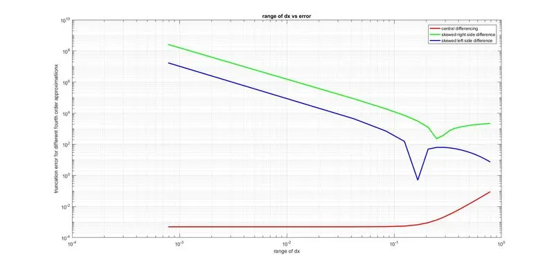
from the above graph, it is clear that the central difference approximation has less error compared to the left and right-skewed approximation.
the cd scheme collet the data from the both side , when the points at extreme we can't use CD but skewed approximations can be used