Week 4.1 - Genetic Algorithm

AIM: TO WRITE A CODE IN MATLAB TO OPTIMIZE THE STALAGMITE FUNCTION AND MAXIMIZE THE GLOBAL MAXIMA

OBJECTIVES:

1. EXPLANATION OF GENETIC ALGORITHM AND SYNTAX IN MATLAB.
2. MAKE SURE THE PROGRAM GIVES THE SAME OUTPUT FOR ANY NO. OF ITERATIONS.
3. PLOTTING ALL THREE GRAPHS(bounded inputs, unbounded inputs & bounded inputs with modified population size), F-MAXIMA VS NO. OF ITERATIONS WITH TITLE, LEGEND, AXES 7 LABELS.

GENETIC ALGORITHM: IT IS BASED ON THE EVOLUTION THEORY PROPOSED BY THE CHARLES DARVIN.

this technique is used for solving both constrained and unconstrained optimization problems, based on natural selection, the process that runs the biological evolution. it constantly changes the population size of the individual solutions.

it always uses three main rules

1. selectin rule
2. cross over rule
3. Mutation rule

in the selection rule, it selects the individuals that contribute to the population at the next generation.

in cross-over rule, it combines two individuals to form the children for the next generation.

in mutation rule, it applies random changes to individual parents to form children.

generally, the genetic algorithm uses in

Optimization, ga is mainly used for optimization, wherein a given set of constraints we have to maximize or minimize the objective function.

Economics, for characterizing the economical model

Neural network, it uses to train recurrent neural networks.

Image processing. for digital image processing and as well as dense pixel matching.

[x,fval,exitflag,output,population, score]=ga(func,nvars,A,b,Aeq,Beq,lb,ub,nonlcon,intcon,options)

where

xis optimum solution

exitflag indicates reason genetic algorithm is stopped

output is info about the optimization process

population- final population

scores-final scores

fun-fitness

nvars-no.of variables

A,b-linear inequality constraints

Aeq,Beq-linear equality constraints

lb-lower limit bound

ub-upper limit bound

nonlcon-use of nonlinear constraints

intcon- to get sol integer

options-to get population size minimized with non-default options.

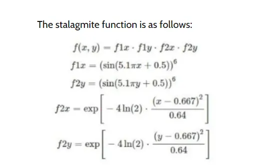
stalagmite function

clear all                 %close all temporary file 
close all                 %closes all the graphs
clc                       % clear command window
% writing optimization program
x=linspace(0,0.6,150);  %defining range of x
y=linspace(0,0.6,150);  %defining range of y

% creating 2d mesh

[xx, yy]=meshgrid(x,y); 

% evaluating stalagmite function

for i=1:length(xx)                  %definig the length of i 
    for j=1:length(yy)               %definig the length of j
        input_vector(1)=xx(i,j);
        input_vector(2)=yy(i,j);
        f(i,j)=stalagmite_function(input_vector); % calling stalagmite function
    end
end
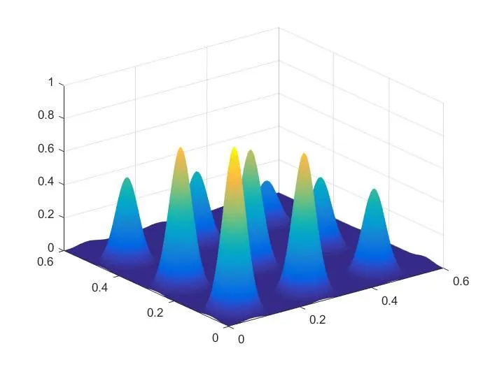
surf(xx,yy,-f);
shading interp;
[x,fval]= ga(@stalagmite_function,2);  % ga function used to run stalgmite data and 
                                        give optimal solution

% unbounded solution program
clear all                 %close all temporary file 
close all                 %closes all the graphs
clc                       % clear command window
% writing optimization program
x=linspace(0,0.6,150);                  %defining range of x
y=linspace(0,0.6,150);                  %defining range of y

% crerating 2d mesh
[xx, yy]=meshgrid(x,y);

% for evaluating stalagmite function
for i=1:length(xx)                      %definig the length of i 
    for j=1:length(yy)                   %definig the length of j
        input_vector(1)=xx(i,j);
        input_vector(2)=yy(i,j);
        f(i,j)=stalagmite_function(input_vector);  % calling stalagmite function
    end
end
surf(xx,yy,-f);
hold on
shading interp;                                  % to make the plot look smoother

% unbounded
tic                                             % study time start
num_cases=50;                                   % GA runs for 60 iteriations
for i=1:num_cases
    [results, fopt(i)]=ga(@stalagmite_function, 2); calling GA function
    xopt(i)=results(1);
    yopt(i)=results(2);
end
study_time1=toc                                  % study time ends
figure(2);

subplot(2,1,1)
hold on
surfc(xx, yy, -f);                              % generation of stalagmite function
shading interp;                                  % to get make the plot smoother

plot3(xopt,yopt,-fopt,'marker','o','markersize',5,'markerfacecolor','r');
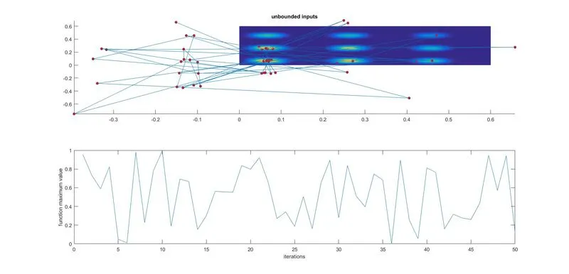
title('unbounded inputs');
subplot(2,1,2);
plot(-fopt);                                    % plot values for every iteration
xlabel('iterations');
ylabel('function maximum value');



%% bounded solution program
clear all                 %close all temporary file 
close all                 %closes all the graphs
clc                       % clear command window

x=linspace(0,0.6,150);        %defining range of x    
y=linspace(0,0.6,150);        %defining range of y

% crerating 2d mesh
[xx, yy]=meshgrid(x,y);

% for evaluating stalagmite function

for i=1:length(xx)                  % defining length of i
    for j=1:length(yy)               % defining length of j
        input_vector(1)=xx(i,j);
        input_vector(2)=yy(i,j);
        f(i,j)=stalagmite_function(input_vector);   % calling stalagmite function
    end
end
surf(xx,yy,-f);       % generation of stalagmite function                              
hold on
shading interp;       % to make the plot look smoother
tic                   %study time count start
num_cases=50;         %ga runs for 60 iterations
for i=1:num_cases
                      % calling GA function
    [results, fopt(i)]=ga(@stalagmite_function, 2, [],[],[],[],[0,0],[0.6,0.6]); 
    xopt(i)=results(1);
    yopt(i)=results(2);
end
study_time1=toc;      % study time count stop 
figure(2);
subplot(2,1,1)
hold on
surfc(xx, yy, -f);    % generating stalgmite function 
shading interp;        5 to make the plot look smoother
plot3(xopt,yopt,-fopt,'marker','o','markersize',5,'markerfacecolor','r');
title('bounded inputs');
subplot(2,1,2);
plot(-fopt);         % plotting value for every iteration
xlabel('iterations');
ylabel('function maximum value');



%% writing optimization program
clear all                 %close all temporary file 
close all                 %closes all the graphs
clc                       % clear command window

x=linspace(0,0.6,150);        %defining range of x    
y=linspace(0,0.6,150);        %defining range of y

% creating 2d mesh

[xx, yy]=meshgrid(x,y);

% for evaluating stalagmite function
for  i=1:length(xx)                  % defining length of i
    for j=1:length(yy)               % defining length of j
        input_vector(1)=xx(i,j);
        input_vector(2)=yy(i,j);
        f(i,j)=stalagmite_function(input_vector); % calling stalagmite function
    end
end
surf(xx,yy,-f);                  %generation of stalagmite function
hold on
shading interp;                  % to make the plot look smoother

% optimization 
options=optimoptions('ga');
options=optimoptions(options,'populationsize',200)
tic                             % study time count starts
num_cases=50;                   % ga runs for 60 times
for i=1:num_cases                
                       % calling ga function
     [results, fopt(i)]=ga(@stalagmite_function, 2, [],[],[],[],[0,0],[0.6,0.6],[],[],options);
    xopt(i)=results(1);
    yopt(i)=results(2);
end
study_time1=toc;       % studt time count stops
figure(3);
subplot(2,1,1)
hold on
surfc(xx, yy, -f);     % generation of stalagmite function
shading interp;        % to make the plot look smoother
plot3(xopt,yopt,-fopt,'marker','o','markersize',5,'markerfacecolor','r');
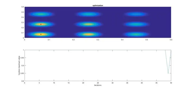
title('optimization');
subplot(2,1,2);
plot(-fopt);           % to  plot values for every iteration
xlabel('iterations');
ylabel('function maximum value');



%% stalgmite function code
function [f]=stalagmite_function(input_vector);
x=input_vector(1);
y=input_vector(2);
f1=(sin(5.1*pi.*x+0.5)).^6;
f2=(sin(5.1*pi.*y+0.5)).^6;
f3= exp(-4*log(2).*(x-0.0667).^2/0.64);
f4= exp(-4*log(2).*(y-0.0667).^2/0.64);

f=-(f1.*f2.*f3.*f4);
end

stalagmite plot

unbounded statistical behavior plot

bounded statistical behavior

optimized plot