Week 5 - Rayleigh Taylor Instability

Aim: Rayleigh Taylor Instability

1) Practical CFD models that have been based on mathematical analysis of Rayleigh Taylor wave.

1) Kelvin-Helmholtz instability

2) Richtmyer- Meshkov instability

3) Plateau-Rayleigh instability

1) Kelvin-Helmholtz instability

Kelvin-Helmholtz instability is an instability at the interface between two parallel streams with different velocities and densities with the heavier fluid at the bottom . In this model, the velocity and density profile are uniform in each fluid layer, but they are discontinuous at the plane interface between the two fluids. This discontinuity in the tangential velocity ie. The shear flow induces vorticity at the interface as a result the interface become an unstable vortex sheet that roll up into a spiral. The heavier fluid parcels from lower denser fluid are lifted up a lighter fluid parcels from lighter upper fluid are pushed down so overall gain potential energy.

2) Richtmyer- Meshkov instability

Instability occurs when two fluid of different density are impulsively accelerated . Normally this is by the passage of shock waves. The development of the instability being s with small perturbation which initially grow linearly with time . This is followed by the non-linear regime with bubbles appearing in the case of light fluid penetrating a heavy fluid and with spikes appearing in the case of heavy fluid penetrating light fluid.

3) Plateau-Rayleigh instability

A liquid jet initially constant radius is falling vertically under gravity . The liquid length increases and reaches a critical value. At this critical value, the jet loses a stream of droplets . This phenomenon occurs primarily as a result of surface tension.

2) Set-up and pre-processing technique for the simulation to carry out.

• Firstly, open the spaceclaim module and select the X-Y plane.
• Select the rectangular geometry and draw 20x20 dimensions on the X-Y axis.
• Take the pul tool to confirm the geometry and moved to new component named as air.
• Again, new component is created under this secondary created component as water with same dimension as shown in below.
• Now these two surface share topology so that we can generate a conformal mesh in meshing module.
• Only one edge was shared from the surface which is connecting both the component.

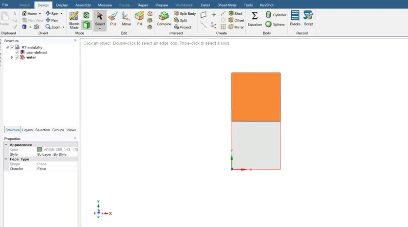
• After the geometry preparation meshing was opened.
• Generate the mesh by providing 0.5mm base mesh size and then proceed with two more case i.e 0.3mm and 0.1mm.

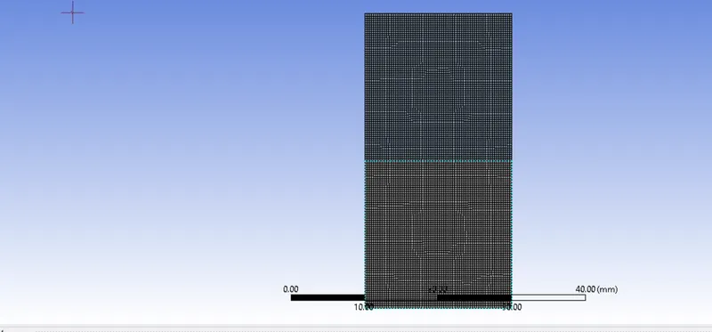
• After meshing fluent was opened.
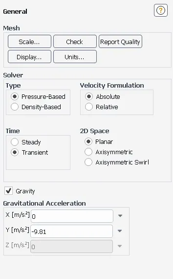
• Defined the transient state and provide the gravity value in y-axis is -9.81m/sq.sec.

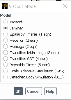
• Select Laminar as a viscous model

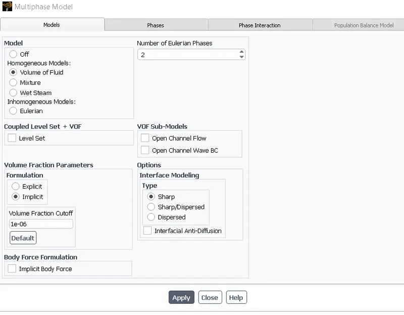
• In multiphase select the viscous of fluid model and implicit formulation.

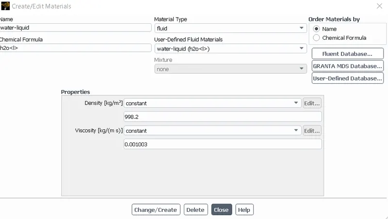
• Select the water-liquid and air form fluent database material and define the air as primary phase and water as a secondary phase by double clicking .

• Now go to the solution module and initialize and case .
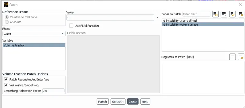
• After that select the patch and patch the case like water->volume of fluid->water surface->1 and then apply.

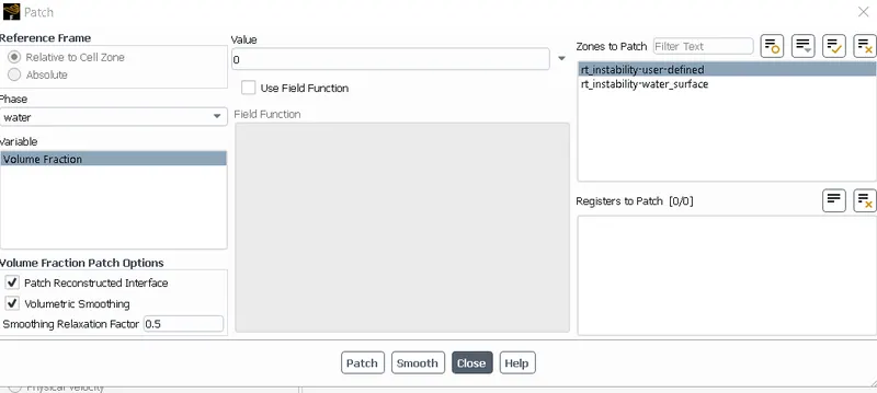
• Repeat the process for air or user-defined surface as well by providing value 0.

• Then go to the result to contour. Select the contour of phase- and phase is water, select all the surface and the save/display.

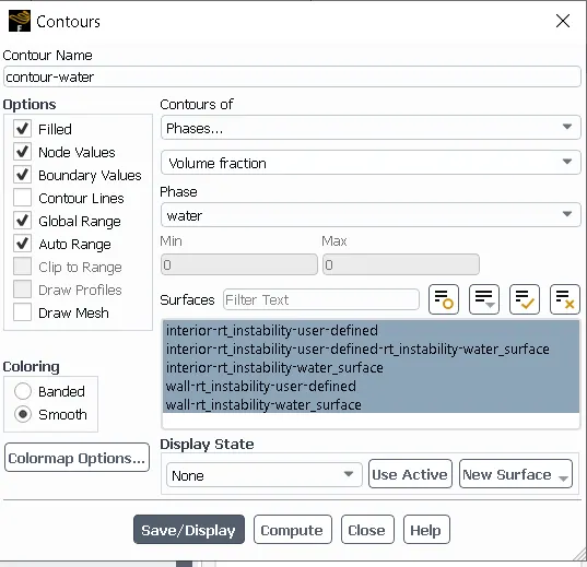
• Now for the the animation select the create in the solution module and then solution animation and create the animation of contour.
• Now finally run the simulation case by adjusting the number of time step and time step size.
• Repeat the same process for the mesh size 0.3mm and 0.1mm and refined mesh.

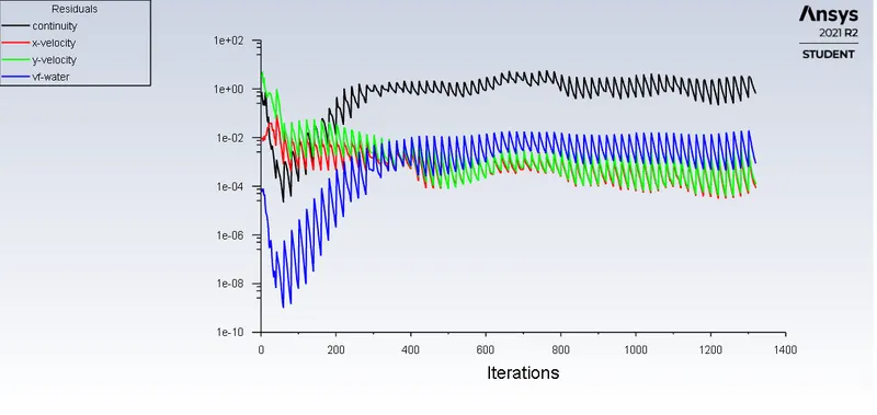
for mesh size 0.5mm

Residuals

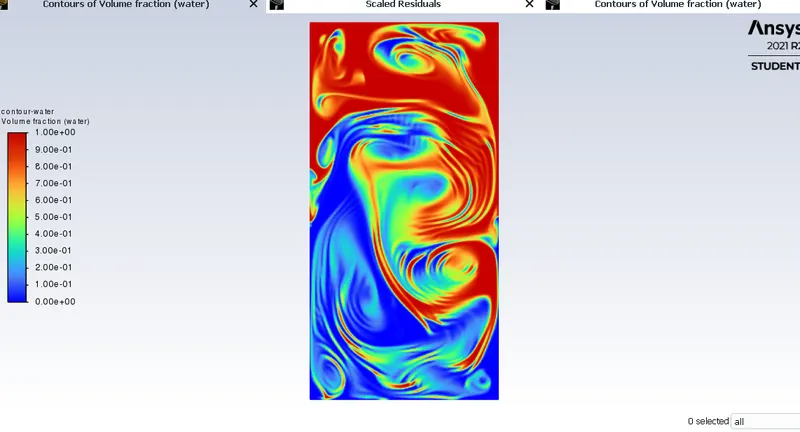
Volume of Fraction

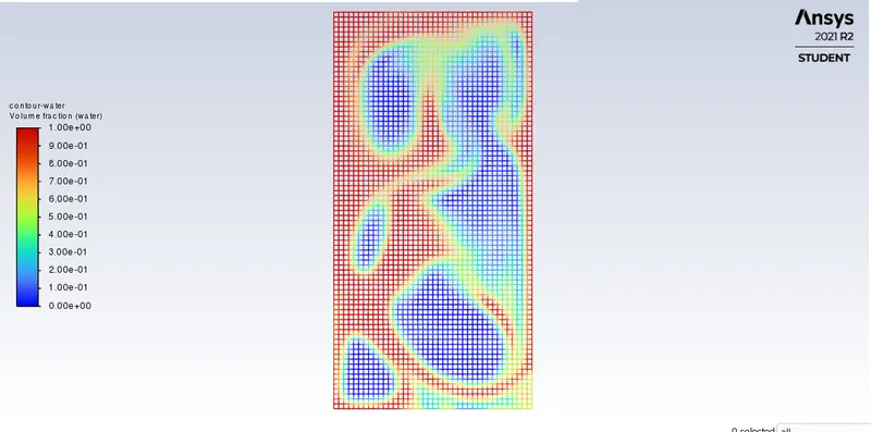
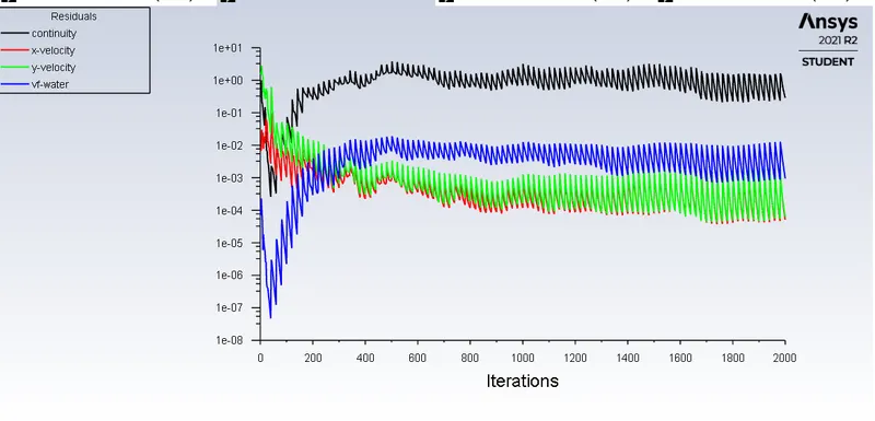
for mesh size 0.3mm

Residuals

Volume of Fraction

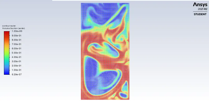
for mesh size 0.1mm

Residuals

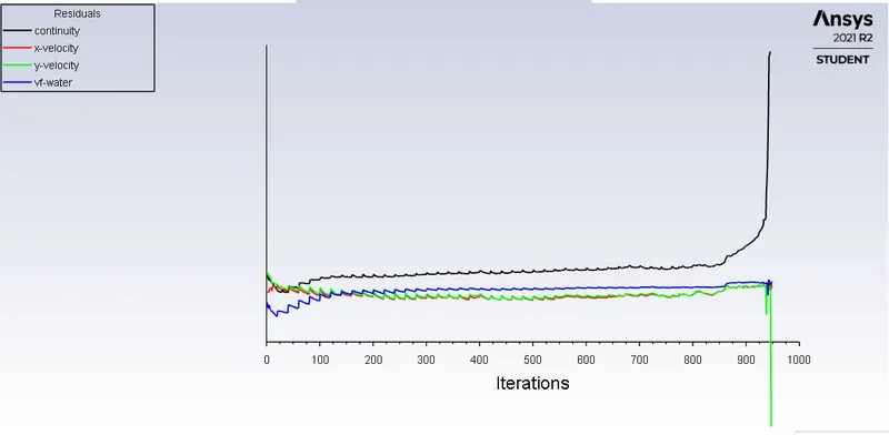
Volume of Fraction

https://youtu.be/M85DIL2aAZ0

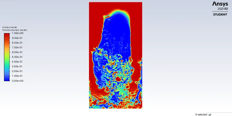
for mesh size 0.1mm and user-defined material

Residuals

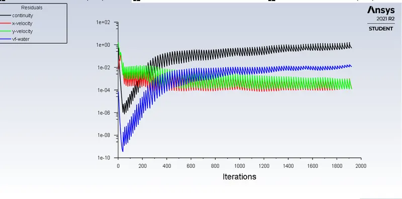
Volume of Fraction

https://youtu.be/LVHlc2V93SU

3) Atwood Number

The Atwood number is the dimensionless number in fluid dynamics used I the study of hydrodynamic instabilities in density stratified flow. It is a dimensionless density ratio defines as :-

A = (X1-X2)/(X1+X2)

X1 = Density of heavier fluid

X2 = Density of lighter fluid

Here in this case, we used water as heavier fluid and air as lighter fluid .

X1 = 1000kg/cubic(m)

X2 = 1.225kg/cubic(m) at STP condition

A = (1000-1.225)/(1000+1.225)

A = 0.997

For user-defined material(Density = 400kg/cubic)

X1 = 1000kg/cubic(m)

X2 = 400kg/cubic(m) at STP condition

A = (1000-400)/(1000+400)

A = 0.428

Hence we can say that lesser the value of Atwood number smoother will be the result.

Result

By comparing all the case we can say that as we go on decreasing the mesh size, the mixing of both fluid will get smoother and more realistic to physical case. Finer the mesh greater the smoothness in the mixing has been achieved.

The Steady state analysis can not be used in this case because in the steady state we focus only on end results but in transient state we have to carried out results and record it for each time step so that we can observe the intermediate behavior of fluids. That’s why transient state analysis is must in this case to capture the intermediate relations and behavior of mixing fluid.

Conclusion

• From above result we can say that, as we decrease the mesh size, smoother will be our contour .
• Here density and viscousity will play the important role in smoothness of result.
• Less density difference material will show more smoother result than other.