Week 5 - Rayleigh Taylor Instability

Aim:

1. To enlist and explain the CFD models that have been based on the mathematical analysis of Rayleigh Taylor waves? To Explain how these mathematical models have been adapted for CFD calculations.
   
   
2. To perform Rayleigh Taylor Instability simulation for baseline and refined mesh using air -water as light and heavy phase pair and onserve the differences in simulation relsults for both meshes. Explain why steady state approach is not suitable for these type of simulations.
   
   
3. To perform Rayleigh Taylor Instability simulation on refined mesh using user define material (`rho = 400 (kg)/m^3` and `mu = 0.001 (kg)/(m*s)`) and water.
   
   
4. To Define the Atwood Number. To find out the Atwood number for both the cases and to explain how the variation in Atwood number in the above two cases affects the behavior of the instability.

1) Rayleigh Taylor Instability:

The instability in case of heavy fluid layer supported by light fluid layer is known as Rayleigh Taylor Instability. It can occur under gravity and equivalently under an acceleration of fluid system in the direction toward the denser fluid. The simplest example is water column supported by air underneath.

Models based on the mathemayical analysis of Rayleigh Taylor Waves:

1. The Kelvin–Helmholtz instability (after Lord Kelvin and Hermann von Helmholtz) is a fluid instability that occurs when there is velocity shear in a single continuous fluid or a velocity difference across the interface between two fluids. Kelvin-Helmholtz instabilities are visible in the atmosphere of planets and moons, such as in cloud formations on Earth or the atmospheres of the Sun and other stars.
   Animation of K-H instability using second order 2D finitevolume scheme.
   
   
   

2. The Plateau–Rayleigh instability, often just called the Rayleigh instability, explains why and how a falling stream of fluid breaks up into smaller packets with the same volume but less surface area. It is related to the Rayleigh-Taylor instability and is part of a greater branch of fluid dynamics concerned with fluid thread breakup. This fluid instability is exploited in the design of a particular type of ink jet technology whereby a jet of liquid is perturbed into a steady stream of droplets

   The driving force of the Plateau–Rayleigh instability is the surface tension of liquids. Liquids tend to minimize their surface area. examples are water dripping from a tap , inkjet printers etc.

   
   
   
   
   
3. The Richtmyer–Meshkov instability (RMI) occurs when two fluids of different density are impulsively accelerated. Normally this is by the passage of a shock wave. The development of the instability begins with small amplitude perturbations which initially grow linearly with time. This is followed by a nonlinear regime with bubbles appearing in the case of a light fluid penetrating a heavy fluid, and with spikes appearing in the case of a heavy fluid penetrating a light fluid. A chaotic regime eventually is reached and the two fluids mix. This instability can be considered the impulsive-acceleration limit of the Rayleigh-Taylor instability.
   
   
   

2) Rayleigh-Taylor instability simulation for air and water material pair:

	Case I (Air and water with baseline Mesh)			Case II (Air and water with refined Mesh):
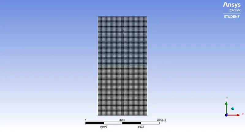
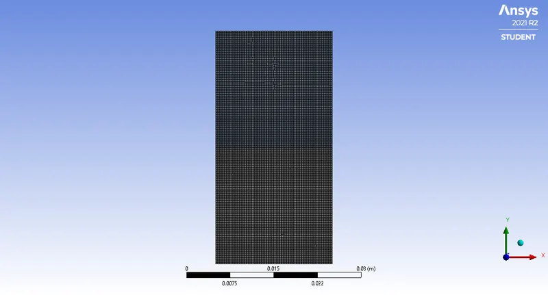
	Mesh: (Mesh size 0.5 mm) No. of elements = 5000.			Mesh: (Mesh size 0.2 mm) No. of elements = 20000.
	Simulation Settings			Simulation Settings
	Solver: Transient Pressure Based solver; Gravity turned on along negative Y directions; Multiphase Model: Volume of fluid; Formulation: Implicit; Primary Phase: air; Secondary Phase: water; with no phase interaction; Time step size:0.005 sec;			Solver: Transient Pressure Based solver; Gravity turned on along negative Y directions; Multiphase Model: Volume of fluid; Formulation: Implicit; Primary Phase: air; Secondary Phase: water; with no phase interaction; Time step size:0.005 sec;
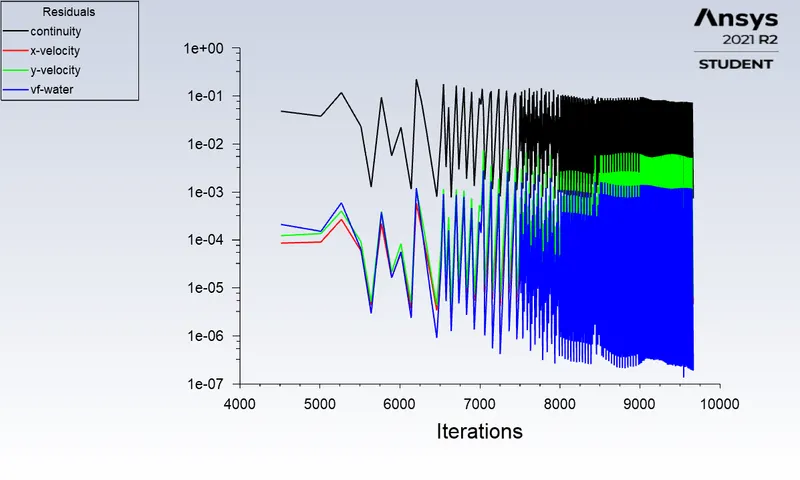
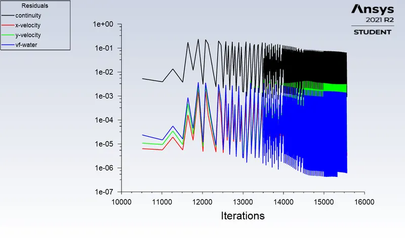
	Residuals Plot			Residuals Plot
	Animation Observations:			Animation Observations:
	The interface is thick as mesh is coarse. The resolution is less and results are smeared out due to coarse mesh. Due to higher Atwood number the bubble and spikes formation is observed.			The interface is thin as mesh is fine. The resolution is high and details of results are captured. Due to higher Atwood number the bubble and spike formation is observed and its details are observed as the mesh is fine.

Animation Case I link:
https://drive.google.com/file/d/1pgv20pieg9gY_twndTw86sDZwONcm752/view?usp=sharing

Animation Case II link:
https://drive.google.com/file/d/1S9C1zRtiUykMVAL0YQy4tRN0vIEU3rhp/view?usp=sharing

The steady state approach does not involve time steps in its solution and generally suitable for final steady state results. As instabilty is time dependent phenomenon and to study the instabilities, the intermediate time step solutions are necessary thus unsteady solvers are used. Thats why steady state approach is not suitable for these type of simulations.

3) Case III (User defined material and water with refined Mesh):

	Case III (User defined material and water with Refined Mesh)
	Mesh: (Mesh size 0.2 mm). No. of elements = 5000.
	Simulation Settings
	Solver: Transient Pressure Based solver; Gravity turned on along negative Y directions; Multiphase Model: Volume of fluid; Formulation: Implicit; Primary Phase: air; Secondary Phase: water; with no phase interaction; Time step size:0.005 sec;
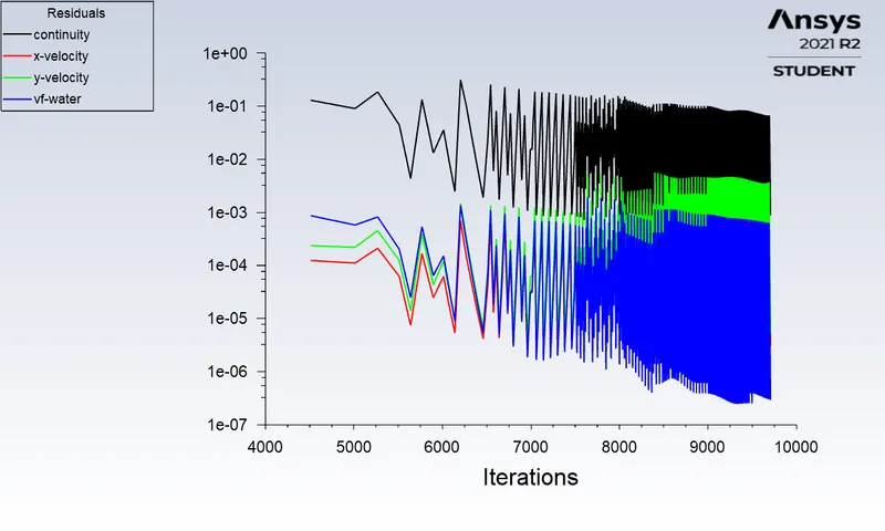
	Residuals Plot:
	Animation Observations:
	The interface is thin as mesh is fine. The resolution is high and details of results are captured. Due to lower Atwood number the nearly symmetric interface disturbance is observed and its details are observed as the mesh is fine. It took higher time evolution of interface disturbance.

Animation Case III link:
https://drive.google.com/file/d/1ZGllBXPAczlXPK13NfmgN7Q7I4h5_B1s/view?usp=sharing

4) The Rayleigh Taylor Instability is typically characterised by the density difference of the two fluids. Thus the dimensionless parameter Atwood Number(`A_t`) is defined, which is the ratio of density difference to the addition of densities.

`A_t = (rho_h - rho_l) / (rho_h + rho_l)`

where `rho_h - "density of heavier fluid" `

`rho_l - "density of lighter fluid" ` .

Atwood numbers play an important role in the study of hydrodynamic instabilities.

		Case I & II	Case III
1	Heavy phase	water	water
	Density of Heavy phase (`(kg)/m^3`)	998.2	998.2
	Viscosity of Heavy phase (`(kg)/(m*s)`)	1.003 e-3	1.003 e-3
2	Light Phase	air	User defined material
	Density of Light phase (`(kg)/m^3`)	1.225	400
	Viscosity of Light phase (`(kg)/(m*s)`)	1.7894 e-5	0.001
3	Atwood Number (`A_t`)	0.9976	0.4278

Obervations based on Atwood number.

It has been observed that the initial density stratification due to compressibility effects which plays a stabilising role while the expansion - compression effect of the flow plays a destabilising role in the Rayleigh Taylor instability.

Hence for lower Atwood number the density difference is small thus density distribution is nearly symmetric along interface thus the initial density stratification plays dominant role while the expansion - compression effect of the flow has less influence.

Similarly for higher Atwood number the density difference is high thus density distribution is asymmetric along interface thus the initial density stratification does not have influence while the expansion - compression effect of the flow plays the dominant role.

Conclusion:

• Thus the Rayleigh Taylor Instability and other details assosiated with the same have been studied and simulation results are in accordance with the theory.