Week 5 - Rayleigh Taylor Instability

Abstract:

The aim of this tudy is simulate a two dimensional Rayleigh taylor imstability problem using Ansys Fluent. Two fluids of two different density are taken for the study. The simulation animation is examined. Different mesh sizes are studied and the ffect of that mesh size on the results are also studied.

key words- Raleigh taylor instability, Ansys, CFD, Multiphase, VOF, patch,Atwood number

Rayleigh taylor instability:

Rayleigh Taylor instabilty is an application of hydrodynamic instabilty occuring between two fluids with different densities . Due to different densities , the two fluids will try to reduce the combined potential energy . The less dense fluid will try to achieve this by forcing its upwards , the dense fluid will try to force down wards.

If the lighter fluid is on top, the interface is said to be stable. If the dense fluid is at top, the interface is said to be unstable in presence of gravity. Examples of thus phenomneon : interstellar gases-Crab Nebulla, mushroom clouds after volcanic eruption.

Atwood number :

This is a dimension less number used in the study of fluid dynamics for studying the hydrodynamic instability in density stratified flows .

`A = (rho(1)-rho(2))/(rho(1)+rho(2))`--1

here , `rho(1)`= density of the heavier fluid

`rho(2)`= density of the lighter fluid.

With air and water , the calculation of Twood number is :

`rho(1)`=1000

`rho(2)`=1.225

So, `A = 0.99755

With an user defined fluid having density 400 kg/m^3;

`A`= 0.4285

Atwood number determines the penetration distance of heavy fluid bubbles into the lighter fluid .

Penetration is a function of `A*g*t^2` , where A is the Atwood number, g is the accleration due to gravity and t is the time .

For the case with air and water , the A is more, so the penetration distance of heavier fluid bubbles into the lighter fluid is more.

• For the Twood number close to 0, the RT instability flow takes the shape of symmetric fingers of fluids.
• For the Atwood number close to 1, the RT instability flow takes the shape of larger bubbles like plumes .

Stages of development :

The evolution of the Rayleigh taylor instability follows four main stages:

In the first stage, the perturbation amplitudes are small when compared to their wavelengths, the equations of motion can be linearized, resulting in exponential instability growth. In the early portion of this stage, a sinusoidal initial perturbation retains its sinusoidal shape.

However, after the end of this first stage, when non-linear effects begin to appear, one observes the beginnings of the formation of the ubiquitous mushroom-shaped spikes (fluid structures of heavy fluid growing into light fluid) and bubbles (fluid structures of light fluid growing into heavy fluid).

At this point, nonlinear terms in the equations of motion can no longer be ignored. The spikes and bubbles then begin to interact with one another in the third stage. Bubble merging takes place, where the nonlinear interaction of mode coupling acts to combine smaller spikes and bubbles to produce larger ones. Also, bubble competition takes places, where spikes and bubbles of smaller wavelength that have become saturated are enveloped by larger ones that have not yet saturated.

This eventually develops into a region of turbulent mixing,which is the fourth and final stage in the evolution. It is generally assumed that the mixing region that finally develops is self-similar and turbulent, provided that the Reynolds number is sufficiently large.

In my analysis the Reynolds number is quite low, so Laminar modelling is considered.

Practical CFD models based on rayleigh Taylor instability :

• Smoother particle hydrdynamics- Smoothed-particle hydrodynamics (SPH) is a computational method used for simulating the mechanics of continuum media, such as solid mechanics and fluid flows. It was developed by Gingold and Monaghen and Lucy in 1977, initially for astrophysical problems. It has been used in many fields of research, including astrphysics, ballistic, volcanology, and oceonography It is a mesh free lagrangian (where the co-ordinates move with the fluid), and the resolution of the method can easily be adjusted with respect to variables such as density.
• Richter-Meyeshkov instability - The Richtmyer–Meshkov instability (RMI) occurs when two fluids of different density are impulsively accelerated. Normally this is by the passage of a shock wave The development of the instability begins with small amplitude perturbations which initially grow linearly with time. This is followed by a nonlinear regime with bubbles appearing in the case of a light fluid penetrating a heavy fluid, and with spikes appearing in the case of a heavy fluid penetrating a light fluid. A chaotic regime eventually is reached and the two fluids mix. This instability can be considered the impulsive-acceleration limit of the rayleigh taylor instability
• Plateau Rayleigh instability- The Plateau Rayleigh instability explains the braeking of falling stream of fluids into smaller packets with same volume but less surface area.

CFD Modelling:

• Geometry preparation
• Mesh generation and refinement
• CFD case set up(Solver set up, multiphase modelling,etc)
• Solution and post-processing

Geometry :

A simple 2D geometry is created in space claim using the sketch option. The dimensons are 0.2 m length and breadth for both the liquids. A surface is created out of the 2D sketch using the pull tool in space claim

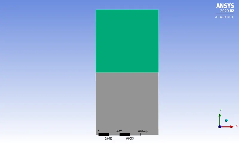
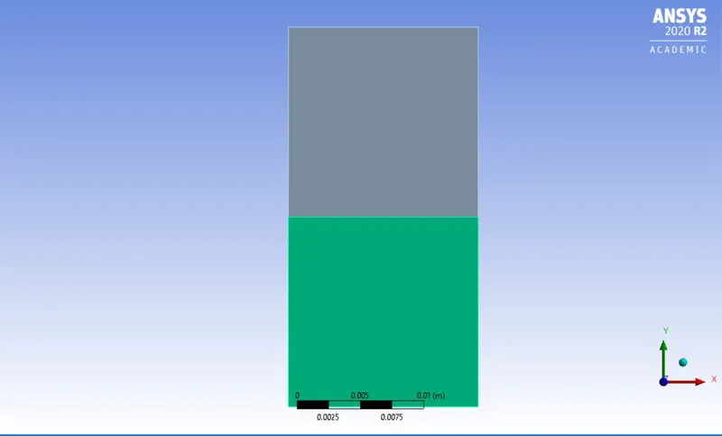
The top surface is for the heavier fluid. the bottom surface is for the lighter fluid.

Meshing:

• Baseline simulation:

Element size	5e-004
Nodes	1891
Elements	1800

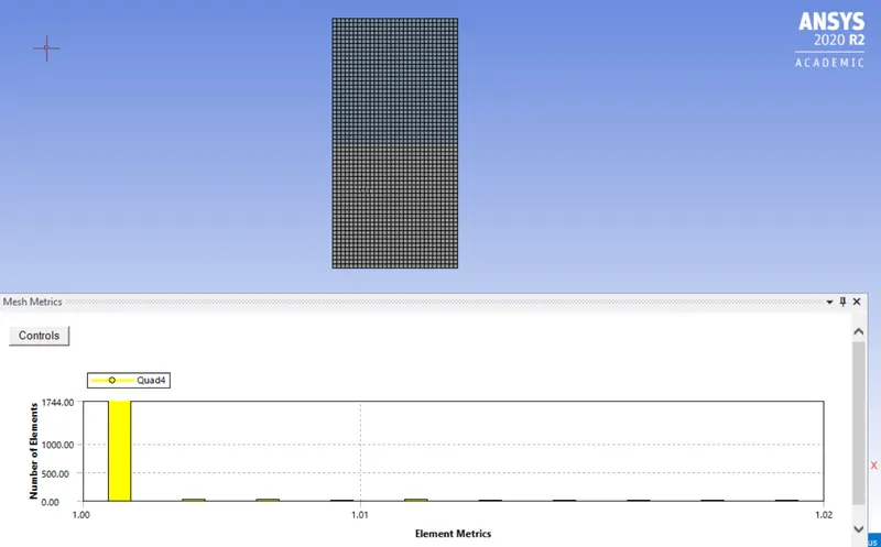
Aspect ratio:

minimum	1
maximum	1.0213
average	1.0003
standard deviation	1.6758e-003

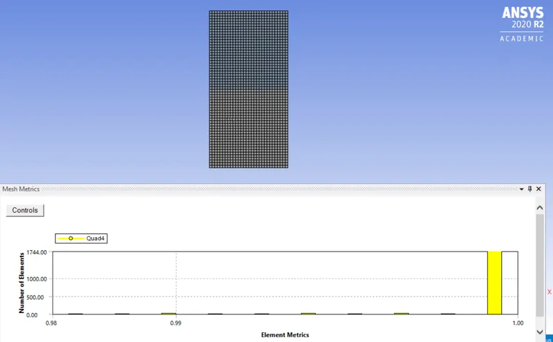
Element quality:

minimum	0.98315
maximum	0.99947
average	0.99922
standard deviation	1.5344e-003

Skewness:

minimum	1.3057e-010
maximum	2.0453e-002
average	3.297e-004
standard deviation	2.0015e-003

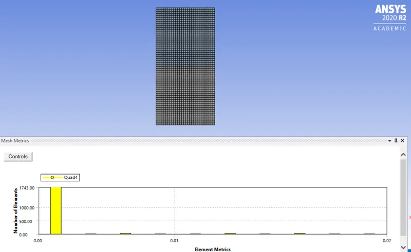
Orthogonal quality:

minimum	0.9949
maximum	1
average	1
standard deviation	3.0859e-005

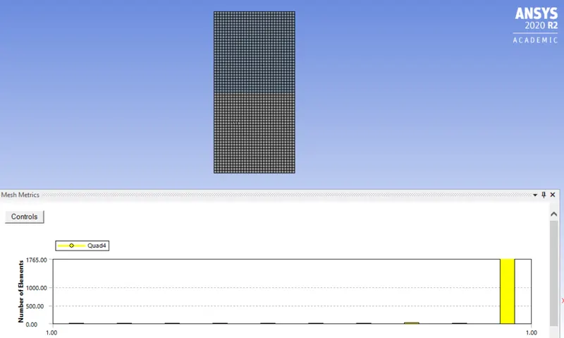
• Refined mesh

element size	3e-4
nodes	5151
elements	5000

Element quality:

minimum	0.98672
maximum	0.99947
average	0.99928
standard deviation	1.06e-003

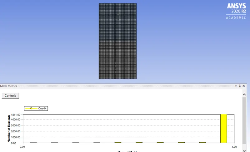
Orthogonal quality;

minimum	0.99971
maximum	1
average	1
standard deviation	1.295e-005

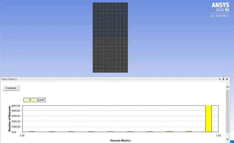
Skewness:

minimum	1.3057e-010
maximum	1.604e-002
average	2.378e-004
standard deviation	1.4653e-003

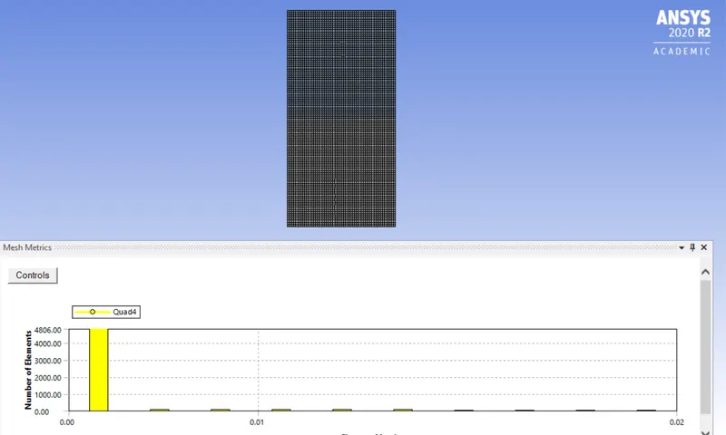
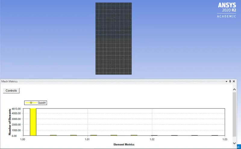
Aspect ratio:

minimum	1
maximum	1.025
average	1.004
standard deviation	2.07e-003

• Refined mesh 2 :

element size	0.0001 meters
nodes	45451
elements	45000

Mesh quality:

Element quality:

minimum	0.9767
maximum	0.99947
average	0.99895
standard deviation	2.11886e-003

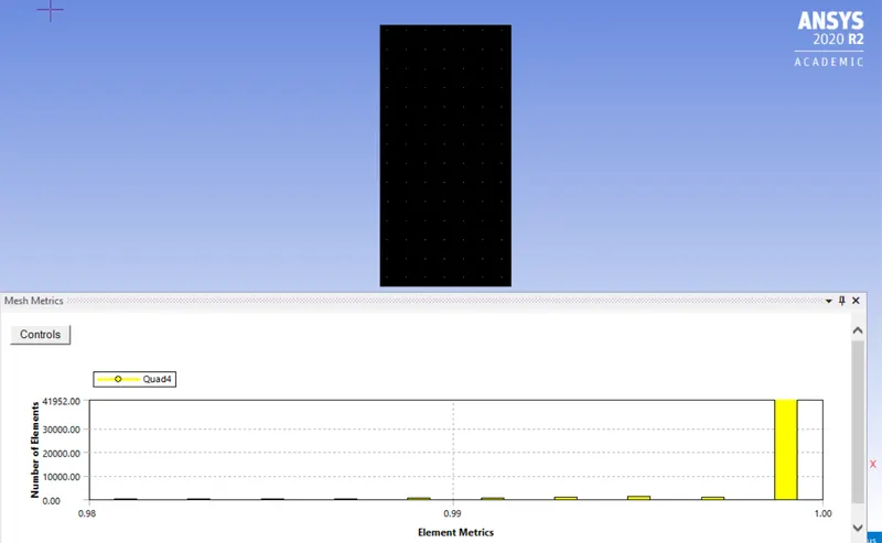
Skewness :

minimum	1.3057e-010
maximum	3.0257e-002
average	7.0065e-004
standard deviation	2.7714e-003

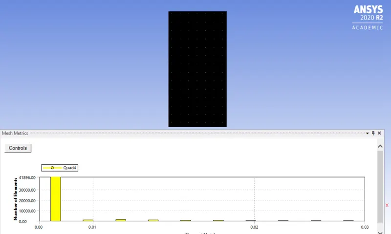
Aspect ratio:

minimum	1
maximum	1.0225
standard deviation	2.0025e-003
avaerage	1.005

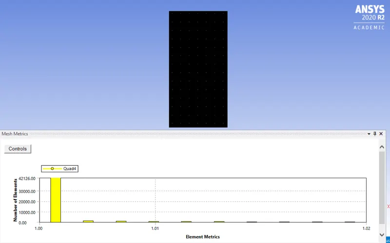
Orthogonal quality:

minimum	0.99901
maximum	1
average	0.9999
standard deviation	4.8442e-005

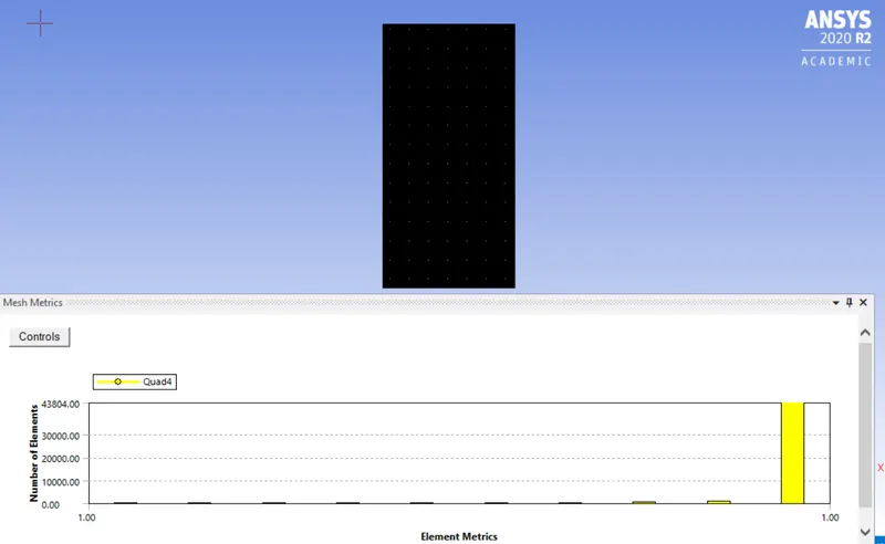
Solution and physics set up:

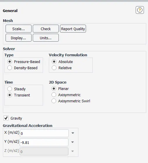
• General settings:

Pressure based solver used.

Transient analysis is performed.

The gravity plays a role in the simulation, So the gravity is turned on. Along the y axis, a value of -9.81 m/s^2 is set as the 2d geometry is along the x-y plane.

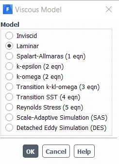
• Viscous model:

The laminar flow is chosen for tha analysis since the velocity of flow is quite low.

• Multiphase model:

In multiphase flows , a phase can be defined as an ientifiable class of material that has a particular inertial response to and interaction with flow and the potential field in which it is immersed.There are two approaches in multiphase modelling: Euler-Euler and Euler-Lagrange. Again Euler-Lagrange has three subdivisions, Volume of fraction, Mixture model and the Euleria model

Volume of Fraction model is the method for this simulation. It is a surface tracking technique applied to a fixed Eulerian mesh. It is desigmed for two or more immiscible liquids whre position of interphase btween the fluids is of interest.

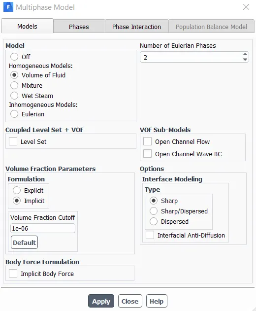
Since the domain constitute of two phases, Multiphase modelling needs to be done, In the model section, Volume of fluids is selected. The formulation i opted for is implicit. Explicit formulation may lead to courant number shooting beyond the prescribed limit ,which is bad. The volume cut off limit is 1e-6. Number of eulerian phase is 2.

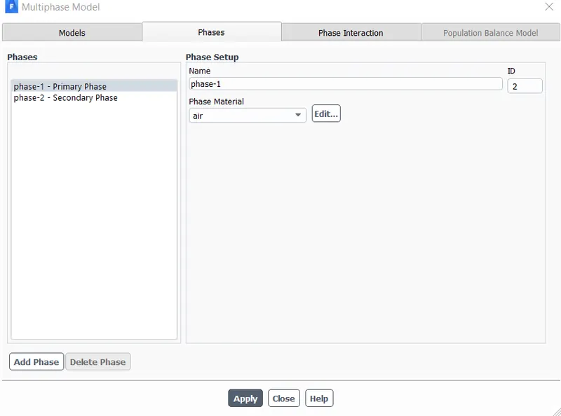
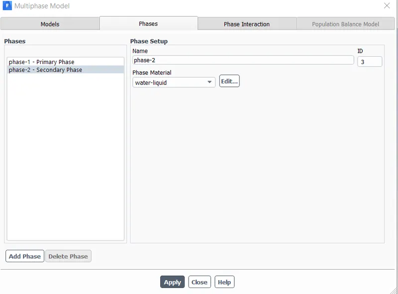
In the phases section, Proper phases needs to be selected. The primary phase is Air that is phase 1, The secondary phase is water, that is phase 2.

The water can be opted for from the fluent database.

Standard initialisation is done .

Patch:

After the initialisation, patch should be created. The basic idea of patching is assigning a volume fraction to certain zones . Here the secondary phase and the water zone is patched 1 agains volume fraction of water , and the other zone is patched 0.

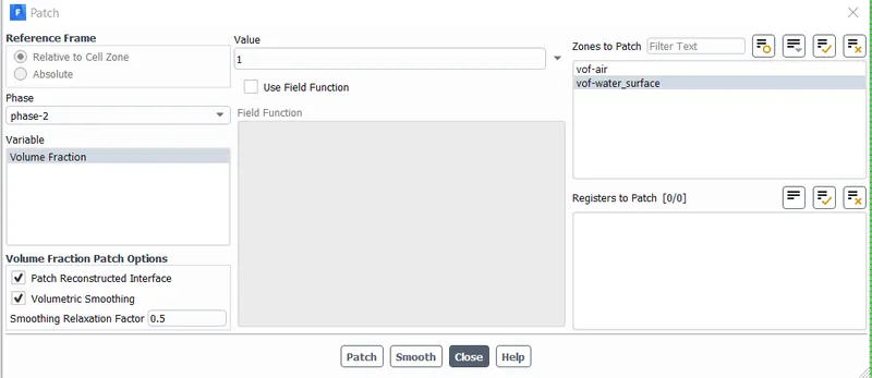
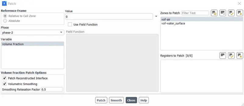
When the zone patched is water surface then the value is set to 1, when the zone patched is air surface , the value is set to 0.

The solution method selected are :

The pressure velocity coupling xcheme is SIMPLE

First order upwind is chosen for the momentum .

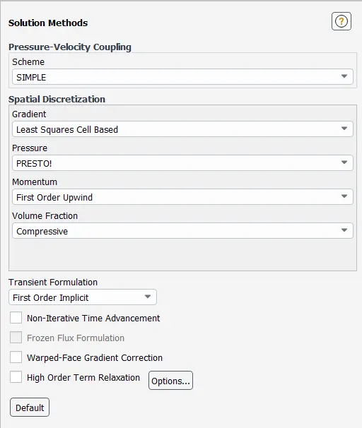
The time step size chosen is 0.005 and the number of time steps is 1000. The residual plot and the contours are studied.

• Results:

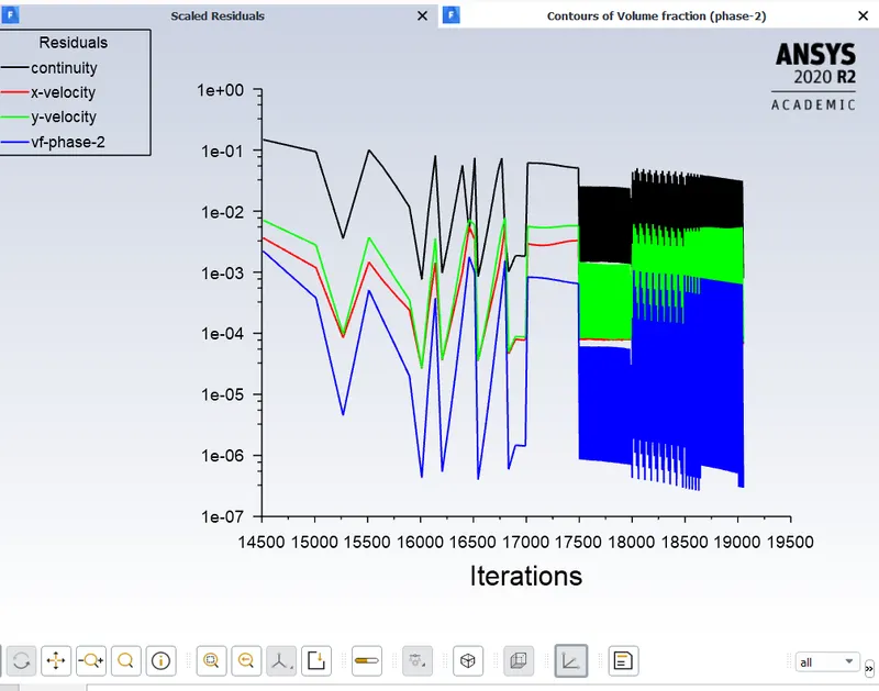
Residuals for the simulation with three mesh sizes starting from initial mesh of 0.0005 meters , 0.0003 meters and 0.0001 meters are pasted below.

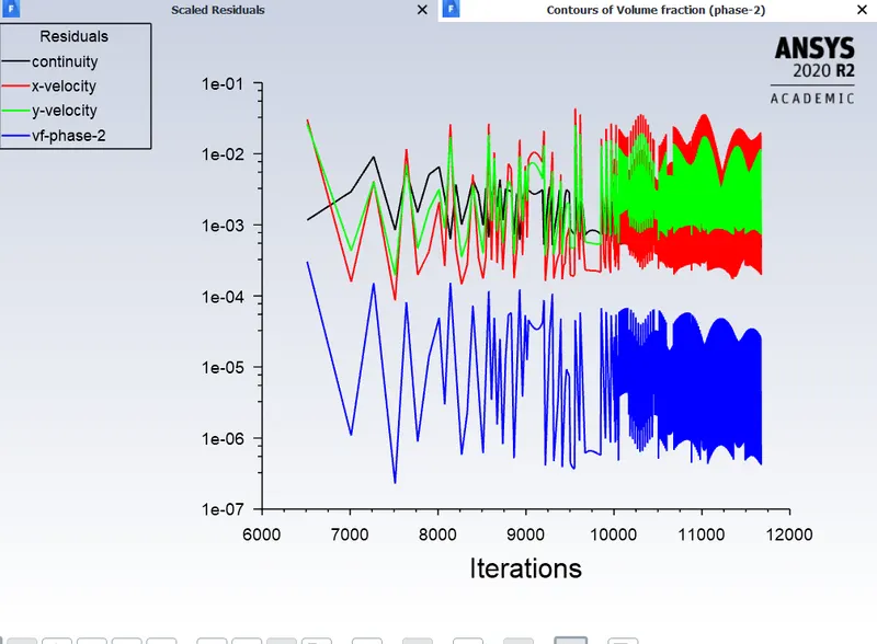
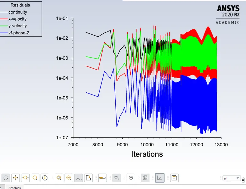
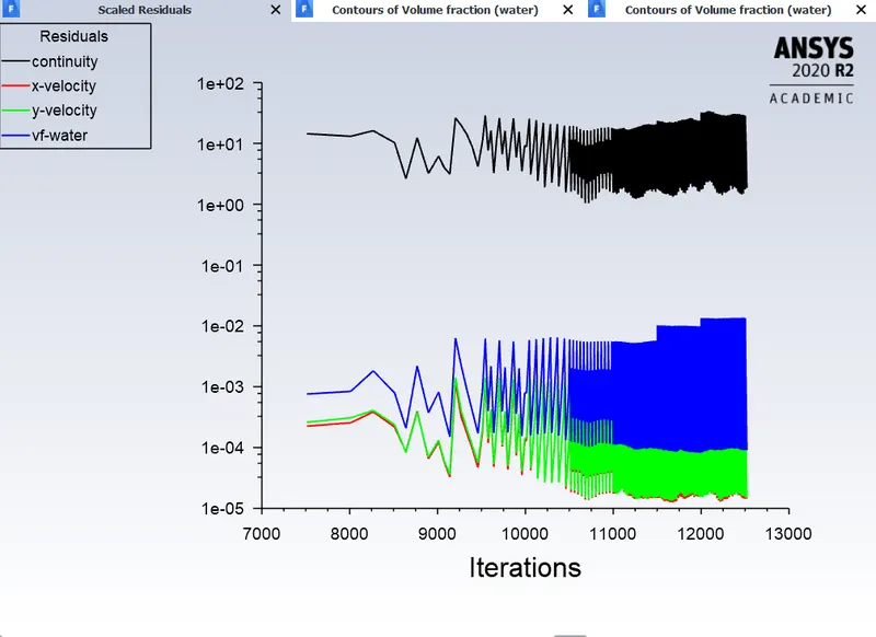
The simulation with finest mesh size convergerd at higher residuals.

The google drive links for the simulations are provided below. Here the animations are created at each 10 time steps.

https://drive.google.com/drive/folders/1DZVc5GwhS60lzHY-HT4fVjbCtka2P-8_?usp=sharing

The final snippets of the simulations are pasted below for mesh size 0.0005 meters,0.0003 meters and 0.0001 meters

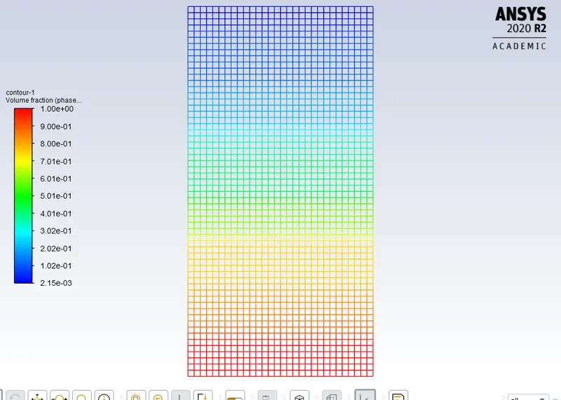
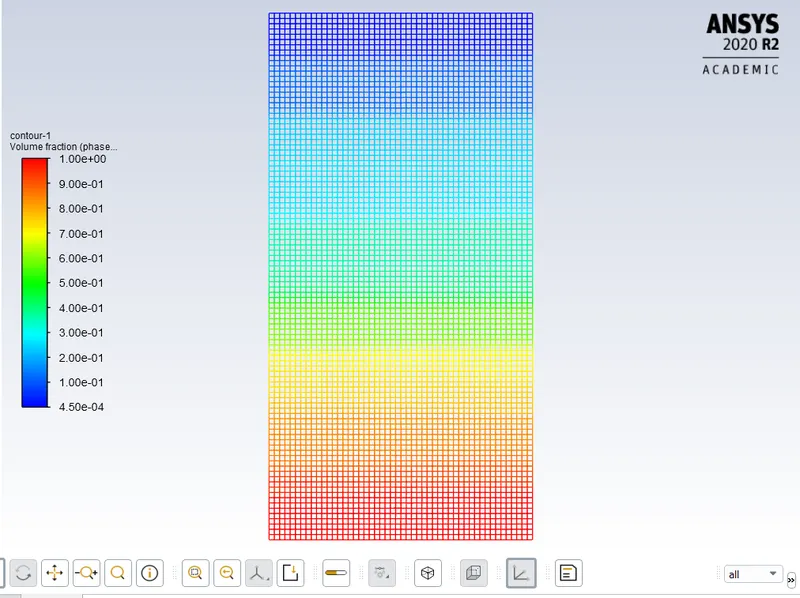
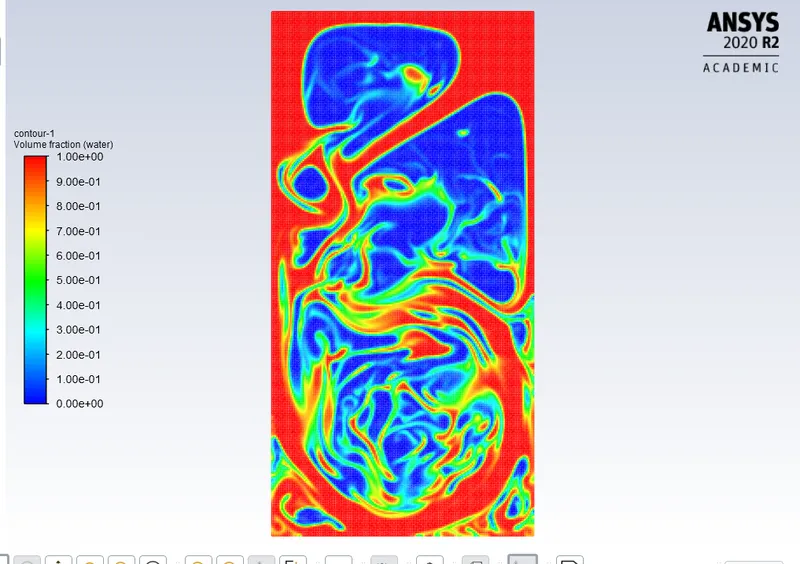
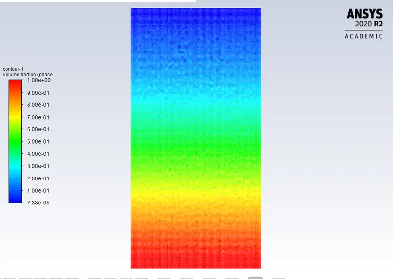
An user defined fluid is created with density 400 kg/m^3 and viscosity 0.001 . The primary phase is the lighter liquid that is the user defined fluid and the secondary fluid is the water. Procedure followed is same. number of time steps is 1000 and the time step size is 0.005. The scaled residual and the snippet is pasted below:

The animation is already there in the google drive link provided.

• Conclusion:

With the finer mesh the finger like penetration and the bubble formation is much more pronounced.

The Atwood number for air-water modelling is 0.9975 and for water-user defined fluid is 0.42. Since the Atwood number is close to 0 in water-user defined fluid simulation, the instabilities are in the form of finger like structures. Since the Atwood number is close to 1 in the air-water simulation the perturbations are in the shape of bubbles.

The RT instability is studied for a 2D case .