Week 5 - Rayleigh Taylor Instability
AIM:
- To find some practical CFD models that have been based on the mathematical analysis of Rayleigh Taylor waves.
- To perform the Rayleigh Taylor instability simulation for 2 different mesh sizes with the base mesh being 0.5 mm and comparision of results.
- Defining atwood number and explain the variation of atwood number in two cases that affect the behavior of instability.
Rayleigh Taylor Instability (RTI) is a phenomenon that occurs at the interface of fluids of different density wherein the lighter fluid pushes the heavier fluid due to the density difference. It is a dynamic process wherein the system tries to reduce its combined potential energy. Examples include the behavior of water suspended above oil in the gravity of Earth, mushroom clouds like those from volcanic eruptions and atmospheric nuclear explosions, supernova explosions in which expanding core gas is accelerated into denser shell gas, instabilities in plasma fusion reactors etc.
CFD models based on mathematical analysis of Rayleigh Taylor waves:
1. Mass diffusion model:
The mass diffusion equation describes the transport of mass and energy due to model viscosity and hence drives actual mixing in the fluids. Even if any configuration is Rayleigh-Taylor unstable, the diffusion process could be responsible for significant mixing if the viscosity is sufficiently large.
2. Single fluid model:
2.1. Potential flow model
This model is valid for all instability changes from the linear stage through the early non-linear to the asymptotic but limited to Atwood number = 1. In this model, single-mode perturbation expands the flow equations to second-order around the bubble tips, hence obtaining an ordinary differential equation for the bubble velocity.
2.2. Buoyancy drag model
It is valid for every Atwood number but limited to the non-linear stages of the instability. It uses ordinary differential equations to evolve the width of the mixing layer. The bubble, or spike, amplitudes are described by balancing the inertia, buoyancy and drag forces. These models cannot model multiple mixing interfaces; cannot be easily extended to 2 or 3 dimensions, and as a rule, do not address demixing, also known as counter gradient transport, i.e. reduction of total fluid masses within the mixing zone. To address the above problems, two-fluid(or multi-fluid)models have to be used.
2.3. Besnard-Harlow-Rauenzahn(BHR)
It is a more advanced version of the single-fluid model. The BHR model is based upon the evolution equations arising from second-order correlations and gradient-diffusion approximations. Using a mass-weighted averaged decomposition, the original BHR model includes full transport equations for the Reynold stresses, turbulent mass-flux velocity, density fluctuations, and the turbulent kinetic energy dissipation rate.
3. Multi-Fluid model:
These models use a separate set of equations for each fluid in addition to the main flow equations and provide an accurate modeling framework for demixing by correctly capturing the relative motion of the different fluid fragments.
The first step for the development of turbulence models is to perform Reynold averaging of the governing equations and resultant terms.
3.1. Two equation K-L turbulence model:
The K-L turbulence model involves equations for turbulent kinetic energy K and turbulent length scale L. The starting point for deriving the model equations are the buoyancy-drag models for the self-similar growth of RT instabilities.
3.2. Three-equation K-L-a turbulence model:
The three equation model was developed as an extension to the two-equation K-L model by including a third equation for the turbulent mass-flux velocity.
3.3. Four-equation K-L-a-b turbulence model:
The four equation model was developed as an extension to the three-equation K-L model by including a fourth equation for density-specific volume covariance. The model can accurately reflect the effects of the changes in the density fluctuations.
Modelling the Rayleigh Taylor instability:
Pre-Processing:
Step 1: Preparation of geometry
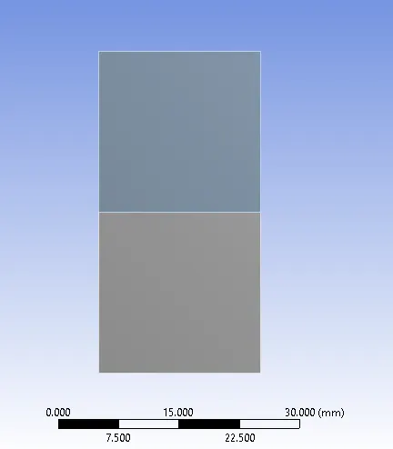
The geometry is essentially two squares , one on top of another of side 20 mm. The top square is assigned the fluid water domain and the bottom domain is assigned the lesser denisity fluid which is air in this case . The common edge between the domains was shared using share tool in Workbench. The created geometry is depicted below:
Meshing:
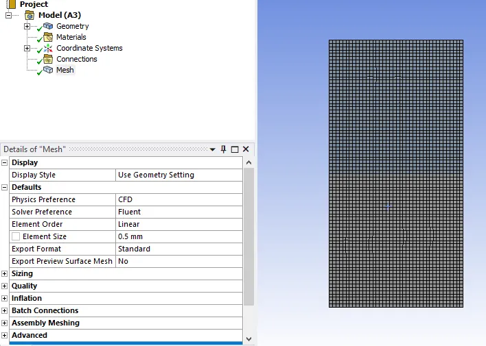
case 1) A baseline mesh with a default element size of 0.5 mm is created as shown below:

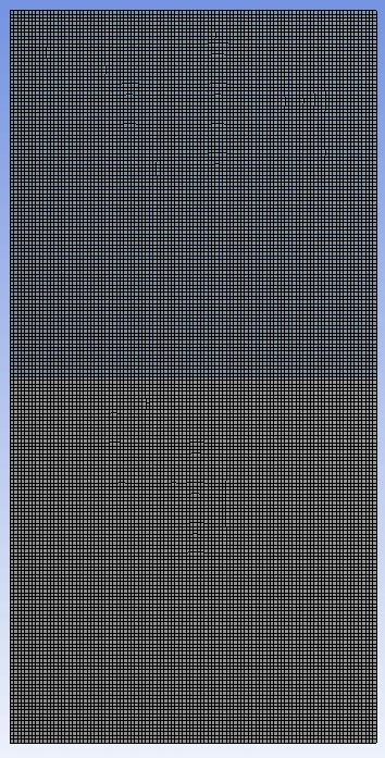
case 2) A refined mesh with an element size of 0.2 mm and the statistics are shown below:

Physics setup on ANSYS Fluent:
A Pressure based , transient solver with Absolute velocity formulation with acceleration due to gravity of 9.81 `m/s^2` enabled in the negative y direction.
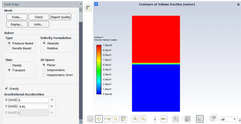
A multiphase model with volume of fluid is chosen to have two different eulerian phases with implicit formulation.
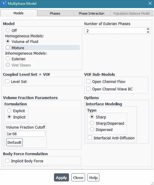
A primary phase of air is chosen and a secondary phase of water liguid is chosen. Later for the refined mesh, a user defined material with (density = 400 kg/m3, viscosity = 0.001 kg/m-s) is chosen to analyze and compare the results.
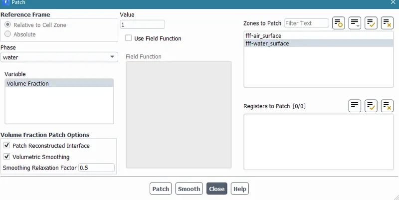
After a standard hybrid initialization, we need to patch both the domains of water and air to the respective materials, wherein the volume-fraction value of 1 to water and 0 to air and (user-defined material).
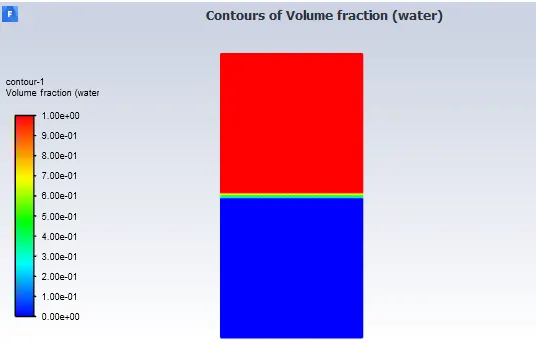
The initial contours for the volume of fraction are shown:
Animation files for different cases are given below:
The animation file for 0.5 mm mesh is given below:
https://drive.google.com/file/d/1dACBAQ0-BRoYJUMZrYMm0y1v0RJZU5IC/view?usp=sharing
The animation for 0.2mm mesh is given below:
https://drive.google.com/file/d/1VfT8g3EVEnWVbtahHSqUuVHqv4qs2Qx2/view?usp=sharing
The animation for user defined material is given:
https://drive.google.com/file/d/1rYQI--c0C46OKUi_Z0kyI9hoPjFSHZwC/view?usp=sharing
Observation:
Finer mesh captures the instability better than the coarse mesh , but it takes more time for the heavier fluid to settle down. So it is computationally expensive but produces results with better accuracy.
Since the simulation involves capturing instabilities which are changing in an unpredictable manner as a function of time , transient approach is preferred over steady state approach. If only the final state results are of concern, a steady-state simulation is preferred. In RT-Instability CFD models, we are more concerned to learn about the transition of the irregularities that starts developing when we pour high dense fluid upon low dense fluid under gravity effect. Using a transient solver along with refined mesh, we can compute the smooth transition of irregularities that takes place at the interface of the fluids.
Atwood Number (A):
It is a dimensionless number that is used to study hydrodynamic instabilities in density stratified flows. In Rayleigh–Taylor instability, the penetration distance of heavy fluid bubbles into the light fluid is a function of acceleration time scale,  where g is the gravitational acceleration and t is the time.
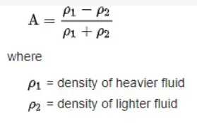
For Air-water RT instability,
`ρ_1` = 998.2 `(kg)/m^3` [Water density]
`ρ_2` = 1.225 `(kg)/m^3` [Air density]
A = (998.2-1.225)/(998.2+1.225)
A = 0.998
For water- UD material RT instability,
`ρ_1` = 998.2 `(kg)/m^3` [Water density]
`ρ_2` = 1.225 `(kg)/m^3` [UD material density]
A = (998.2-400)/(998.2+400)
A = 0.428
Behaviour of RT Instability on variation of Atwood number:
RTI evolves in three distinct stages: Linear stability , mushroom head(falling) or bubble(rising) formation , long term evolution due to bubble merging and mixing. For low Atwood number close to 0, bubble and mushroom head shape is relatively symmetrical, the disturbances or perturbations are linear for a larger time as seen for the user defined material case. In contrast, for large Atwood number, bubble and mushroom head shape is less symmetrical, also it occurs very rapidly at an accelerating rate which leads to a non linear growth rate as seen for the water-air combination.