Week 5 - Rayleigh Taylor Instability
Assignment name-Rayleigh Taylor Instability (ANSYS FLUENT)
Aim-perform simulation of Rayleigh Taylor Instability
Objective-
- perform Rayleigh Taylor Instability Simulation for 2 different mesh with base mesh being 0.5mm (choose air & Water)
- Perform one more simulation with water and user defined material
- Define Atwood number. Find out the Atwood number for both the cases and explain how the variation in Atwood number in the above two case affects the behaviour of the instability
- Why choose transient state over steady state
Introduction Rayleigh Taylor instability
The Rayleigh–Taylor instability is an instability of an interface between two fluids of different densities which occurs when the lighter fluid is pushing the heavier fluid. Water suspended atop oil is an everyday example of Rayleigh–Taylor instability, and it may be modelled by two completely plane-parallel layers of immiscible fluid, the denser on top of the less dense one and both subject to the Earth's gravity. The equilibrium here is unstable to any disturbances of the interface, if a parcel of heavier fluid is displaced downward with an equal volume of lighter fluid displaced upwards, the potential energy of the configuration is lower than the initial state. Thus, the disturbance will grow and lead to a further release of potential energy, as the denser material moves down under the gravitational field, and the less dense material is further displaced upwards.
CFD Models based on Rayleigh Taylor instability:
- Kelvin-Helmholtz instability
Kelvin–Helmholtz instability occurs in the atmosphere as a sporadic, but widespread, phenomenon. It is usually invisible and so can be dangerous as clear air turbulence. The Kelvin–Helmholtz instability typically occurs when there is velocity shear in a single continuous fluid or additionally where there is a velocity difference across the interface between two fluids. A common example is seen with wind blowing over water, the instability constant is able to manifest itself through waves on a water surface. The Kelvin-Helmholtz instability is not only restricted to a water surface as clouds, but is evident through other natural phenomena as the ocean, Saturn's bands and the sun's corona. The theory predicts the onset of instability and transition to turbulent flow within fluids of different densities moving at various speeds.
Helmholtz studied the dynamics of two fluids of different densities when a small disturbance, such as a wave, was introduced at the boundary connecting the fluids. Kelvin-Helmholtz instability can thus be characterized as unstable small-scale motions occurring vertically and laterally.
- Plateau-Rayleigh instability
The Plateau–Rayleigh instability explains why and how a falling stream of fluid breaks up into smaller packets with the same volume but less surface area. It is related to the Rayleigh-Taylor instability and is part of a greater branch of fluid dynamics concerned with fluid thread breakup. This fluid instability is exploited in the design of a particular type of ink jet technology whereby a jet of liquid is perturbed into a steady stream of droplets. The driving force of the Plateau–Rayleigh instability is that liquids, by virtue of their surface tensions, tend to minimize their surface area. A considerable amount of work has been done recently on the final pinching profile by attacking it with self-similar solutions. Liquid dispensers, inkjet printers, and similar spotting systems are designed to induced perturbations (either by means of mechanical oscillations or thermally) in order to ensure correct decomposition of a fluid jet into droplets
- Richtmyer meshkov instability
The Richtmyer–Meshkov instability (RMI) occurs when two fluids of different density are impulsively accelerated. Normally this is by the passage of a shock wave. The development of the instability begins with small amplitude perturbations which initially grow linearly with time. This is followed by a nonlinear regime with bubbles appearing in the case of a light fluid penetrating a heavy fluid, and with spikes appearing in the case of a heavy fluid penetrating a light fluid. A chaotic regime eventually is reached and the two fluids mix. This instability can be considered the impulsive-acceleration limit of the Rayleigh-Taylor instability.During the implosion of an inertial confinement fusion target, the hot shell material surrounding the cold D-T fuel layer is shock-accelerated. This instability is also seen in Magnetized target fusion. Mixing of the shell material and fuel is not desired and efforts are made to minimize any tiny imperfections or irregularities which will be magnified by Richtmyer meshkov instability.
Case 1=material air (density=1.225 kg/m^3 and viscosity=1.7894e-05) and water (density=998.2 kg/m^3 and viscosity=0.001003)
Case2 =material user defined (density=400 kg/m^3 and viscosity=0.001kg/m-s) and water (998.2kg/m^3 and viscosity=0.001003)
**note-case 2 only for finer mesh (element size=0.15mm)
Steps involved in the simulation
Geometry
Mesh
Setup
Solution
Results
Case 1
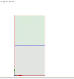
Geometry=it is 2d simulation-geometry is created with two surface namely air and water. Water is the denser fluid at the top. After doing all thing go to workbench (option in space claim) and share the topology
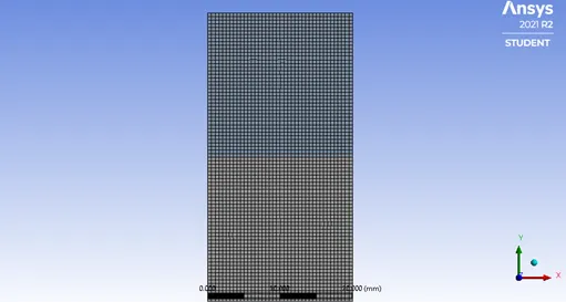
Subcase1 -mesh
Element size=0.5mm
Number of elements=3200
Nodes=3321
setup-
solver type-pressure Based Solver-Transient state
gravity= -9.81 (y-axis)
model-viscous laminar
multiphase-ON
energy-turn off
material properties
fluid-air (density=1.225 kg/m^3)
fluid-water (density=998.2 kg/m^3)
method-Simple
initialization- Standard initialization with patch
solution
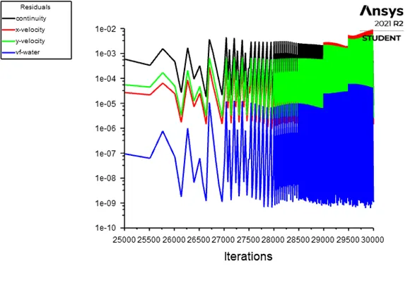
Residual
Volume fraction of water
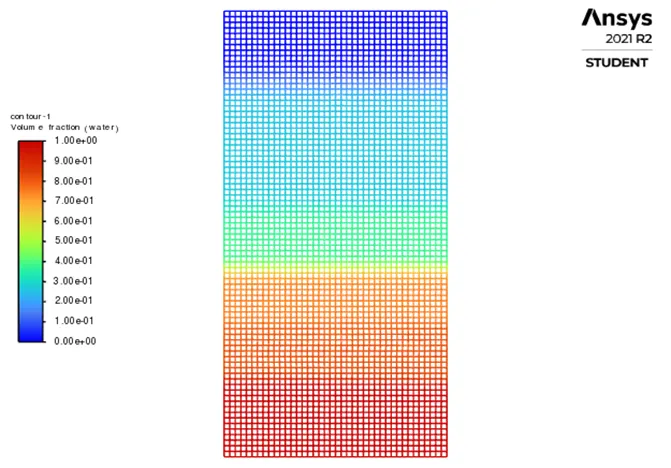
Animation link- https://drive.google.com/file/d/1aU83VY8rA03WhykbyZMcCM4BwVpdbdCj/view?usp=sharing
Subcase 2-
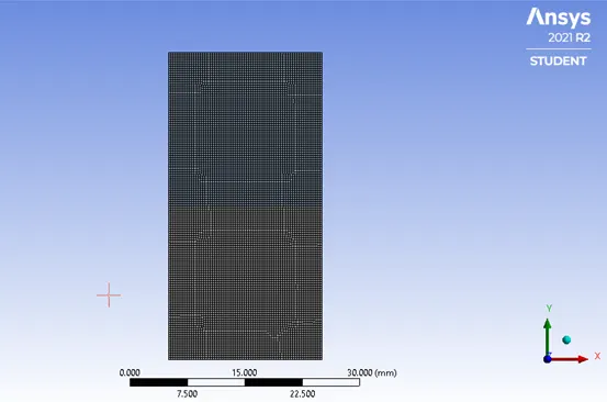
Mesh
Element size=0.3 mm
Number of elements=8978
Nodes=9180
setup-
solver type-pressure Based Solver-Transient state
gravity= -9.81 (y-axis)
model-viscous laminar
multiphase-ON
energy-turn off
material properties
fluid-air (density=1.225 kg/m^3)
fluid-water (density=998.2 kg/m^3)
method-Simple
initialization- Standard initialization with patch
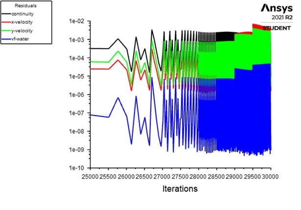
solution
Residual
Volume fraction of Water
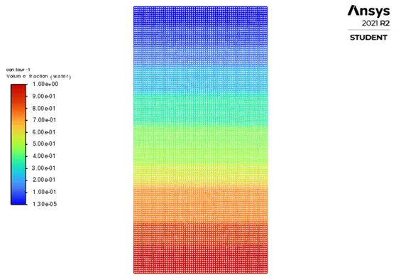
Animation Link- https://drive.google.com/file/d/1iXcNAMSJNJtPxdXk63jPQg3hAYPHT_CV/view?usp=sharing
Subcase3
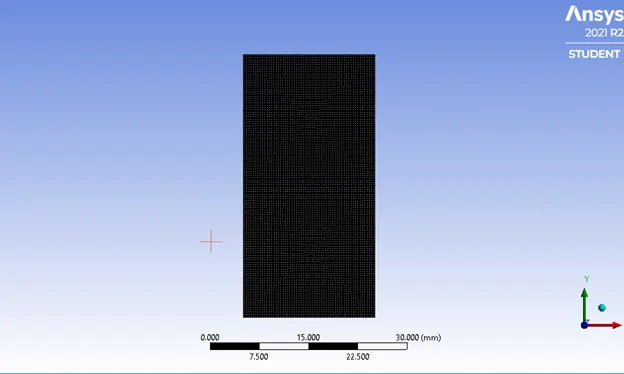
Mesh
Element size=0.15mm
Number of elements=35778
Nodes=35378
setup
solver type-pressure Based Solver-Transient state
gravity= -9.81 (y-axis)
model-viscous laminar
multiphase-ON
energy-turn off
material properties
fluid-air (density=1.225 kg/m^3)
fluid-water (density=998.2 kg/m^3)
method-Simple
initialization- Standard initialization with patch
solution
Residual
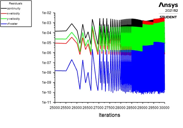
Volume fraction
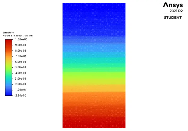
Animation Link- https://drive.google.com/file/d/1ELHQAeBApvfpDZrkkK3RYjGYA48UdOib/view?usp=sharing
Case 2- User-defined
Geometry=It is 2d simulation-geometry is created with two surface namely user defined material and water. Water is the denser fluid at the top. After doing all thing go to workbench (option in space claim) and share the topology
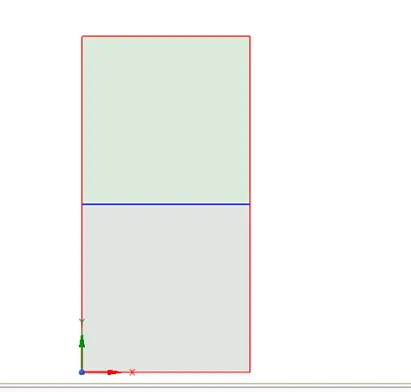
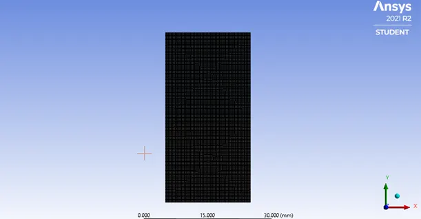
Mesh
Element size=0.15mm
Number of elements=35778
Nodes=35378
setup-
solver type-pressure Based Solver-Transient state
gravity= -9.81 (y-axis)
model-viscous laminar
multiphase-ON
energy-turn off
material properties
fluid-user defined(density=400 kg/m^3, Viscosity=0.001kg/m-s)
fluid-water (density=998.2 kg/m^3)
method-Simple
initialization- Standard initialization with patch
solution
Residual
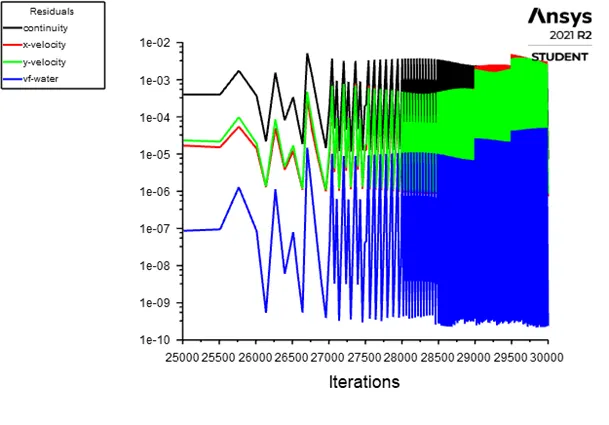
Volume fraction
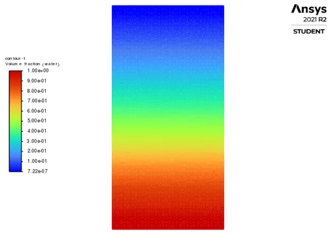
Animation Link-
https://drive.google.com/file/d/1N-jrEBLArBVEtYKm8QAJdM3Uq9sCt9W5/view?usp=sharing
- Atwood number
The Atwood number is a dimensionless number in fluid dynamics used in the study of hydrodynamic instabilities in density stratified flows. It is a dimensionless density ratio related to the density of heavier fluid and the density of lighter fluid. (The difference in the fluid densities divided by their sum). Atwood number is an important parameter in the study of Rayleigh–Taylor instability. For Atwood number close to 0, RT instability flows take the form of symmetric “fingers” of fluid; for Atwood number close to 1, the much lighter fluid “below” the heavier fluid takes the form of larger bubble-like plumes.
Atwood number=(ρ1-ρ2)/(ρ1+ρ2)
Where, ρ1=density of heavier fluid
ρ2=density of lighter fluid
Case 1=material air (density=1.225 kg/m^3 and viscosity=1.7894e-05) and water (density=998.2 kg/m^3 and viscosity=0.001003)
Putting values in above equation we get,
Attwood number=0.997
Case2 =material user defined (density=400 kg/m^3 and viscosity=0.001kg/m-s) and water (998.2kg/m^3 and viscosity=0.001003)
Putting values in above equation we get,
Atwood number=0.4278
-
- Why choose transient state over steady state-
Transient state used because we want to see the behaviour of instability with time and we are not interested in seeing the end results that why choose transient state over steady state
Results-
- As the mesh finer the instability is noticed more prominently and the interference was seen clearly
- Comparison for two cases for finer mesh (element size=0.15mm)
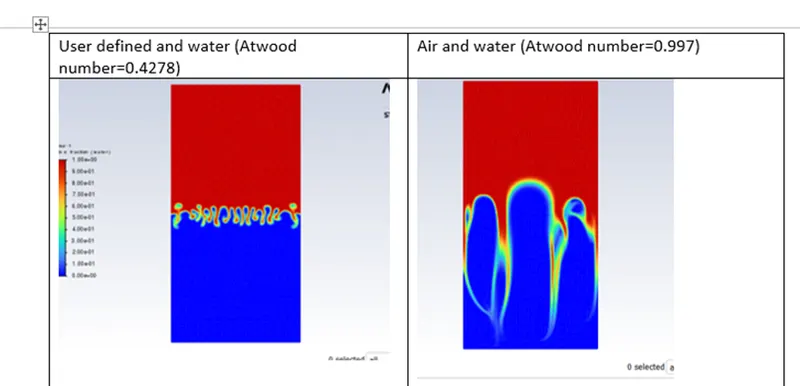
The interface of two fluids was analysed and Atwood number is calculate for two different case maintain in the assignmentsAtwood number close to 0, RT instability flows take the form of symmetric “fingers” of fluid; for Atwood number close to 1, the much lighter fluid “below” the heavier fluid takes the form of larger bubble-like plumes. Form above profiles we can say that our simulation is validate
- The interface of two fluids was analysed and Atwood number is calculated for two different cases
I updated animation after 10 timesteps (total 150 frame)