Week 5 - Rayleigh Taylor Instability

Rayleigh Taylor Instability:-

The Rayleigh Taylor Instability occurs when the interface between two fluids of different densities is such as, lighter fluid is pushing the heavier fluid upward. Initially, two horizontal immiscible fluids, with a sharp interface separating them, lie horizontally with the heavier fluid above the lighter one. Gravity acts downward, and any small disturbance to the interface leads to unstable growth of fingers of the heavy fluid moving downward and bubbles of the lighter fluid moving upward. That contact discontinuity between the two fluids is unstable to disturbances that grow by transforming potential energy to kinetic energy, causing bubbles of the low-density fluid to rise, and spikes of the high-density fluid to sink. When the lighter fluid is above the heavy fluid, the interface becomes stable.

Types of Instabilities and practical CFD models that have been based on the mathematical analysis of Rayleigh Taylor waves:-

1. Kelvin–Helmholtz instability:-

Kelvin-Helmholtz instability typically occurs separating two immiscible fluids by a velocity variance across their interface and waves can be formed at the interfaces. Instabilities of this kind generally occur in nature, two such manifestations are the “wind-over-water” and “clear air turbulence” instabilities. Suppose two parallel streams of inviscid incompressible fluids superposed one above the other and assume that the upper and lower streams have positive and negative velocities, respectively. Since at the interface there is a discontinuity in the velocity which produces vorticity. vorticity induces a velocity in the positive or negative direction in parts of the sheet displaced upwards or downwards. At the undisturbed points of the sine wave, the vorticity induces a rotational velocity which amplifies the wave and causes the instability to grow. As a result, the vorticity sheet results in vortex rolls and eventually develops in a turbulent manner.

[Image source:- Google]

2. Plateau–Rayleigh instability:-

Liquid streams emerging from a nozzle break up rapidly into droplets due to instabilities driven by surface tension, this is known as Rayleigh–Plateau instabilities. A liquid jet, initially of constant radius, is falling vertically under gravity. The liquid length increases and reaches a critical value. At this critical value, the jet loses its cylindrical shape as it decomposes into a stream of droplets. This phenomenon occurs primarily as a result of surface tension. The droplet formation decreases the jet's surface area and hence its free energy. The most common application is in inkjet printing.

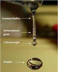
[Image source:- Google]

3. Richtmyer–Meshkov instability: -

The Richtmyer-Meshkov instability occurs if the interface between the fluids is accelerated impulsively rather than continuously, Commonly this is by the passage of a shock wave. The development of the instability begins with small amplitude perturbations which initially grow linearly with time. This is followed by a nonlinear regime with bubbles rising in the case of a light fluid penetrating a heavy fluid, and with spikes appearing in the case of a heavy fluid penetrating a light fluid. In this case, the mismatch in acoustic impedance and the misalignment between the pressure and density gradients lead to both refractions of the shock and the generation of vorticity at the interface, which in turn leads to the growth of the perturbations and the interface distortion. If the shock travels from the hard into the soft fluid, an initial phase reversal takes place, with peaks and troughs trading places along with the interface, followed by the unbounded growth of the perturbations.

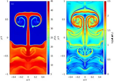
[Image source:- Google]

Practical CFD Models:-

Smoothed particle hydrodynamics (SPH):-

Smoothed particle hydrodynamics is a simple and effective numerical method, that can be used to solve a variety of challenging problems in computational mechanics. In the SPH method, the state of a system is represented by a set of particles, which possesses individual material properties and interact with each other within a specific range defined as a support domain by a weight function or smoothing function. SPH features flexibility in handling complex flow fields and in including physical effects. The advantage of SPH and generally Lagrangian numerical methods over Finite Volume methods is that they do not require a mesh in a classical sense so that they are more suitable for simulations of complex moving geometries. The complexity of modeling the transient gear meshing and the small gap between the gear tooth flanks can be overcome, as no mesh is required for this particle-based approach. The boundary conditions can be modeled by either moving or stationary particles.

Single-Fluid model:-

A typical method used for the analysis of two-phase flows is a mixture model, i.e. the individual fluid phases are assumed to behave as a flowing mixture described in terms of the mixture properties. The applied single-fluid model is a five equation model consisting of the mass, momentum, and energy equations for vapor/liquid mixtures and two equations describing the formation and growth of the liquid phase.

Two-Fluid model:-

A simple version of the two-fluid model is the separated-flow model, in which only one parameter, such as velocity, is allowed to differ between the two phases. Thus the model is expressed in terms of two sets of conservation equations governing the balance of mass, momentum, and energy in each phase. The real significance of the two-fluid model is that it can take into account the dynamic and non-equilibrium interactions between phases. This is accomplished by using the momentum equations for each phase and two independent velocity fields as well as the two energy equations in the formulation. Thus, it is expected that a two-fluid model can be helpful to the analyses of transient phenomena, wave propagations, and flow regime changes. Particularly if the two phases are weakly coupled such that the inertia of each phase changes rapidly, the two-fluid model should be used to study these phenomena.

Turbulence model:-

Turbulence models are needed to predict the average mixing behavior inflows that are on average one or two-dimensional. The approach to the construction of the tile turbulence model is guided by experimental behavior. The equations governing turbulent floes can only be solved directly for simple cases of the floe. For Most real-life turbulent flows, Cfd simulations use turbulent models to predict the evolution of turbulence. These turbulence models are simplified constitutive equations that predict the statical evolution of turbulent flows.

Rayleigh Taylor Instability CFD Simulation Analysis:-

Geometry:-

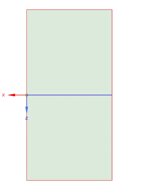
Boundary Conditions:-

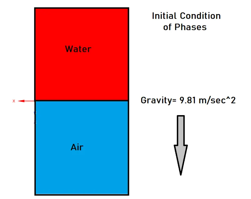
Case Setup:-

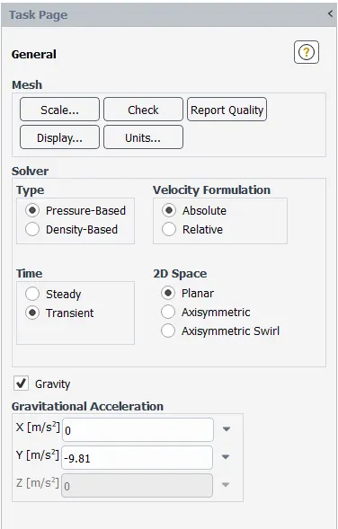
Case-1:-

1. Mesh = 0.5mm

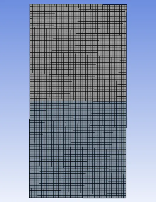
Results:-

Residuals:-

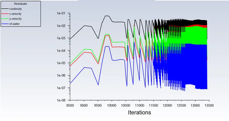
Phases Contour:-

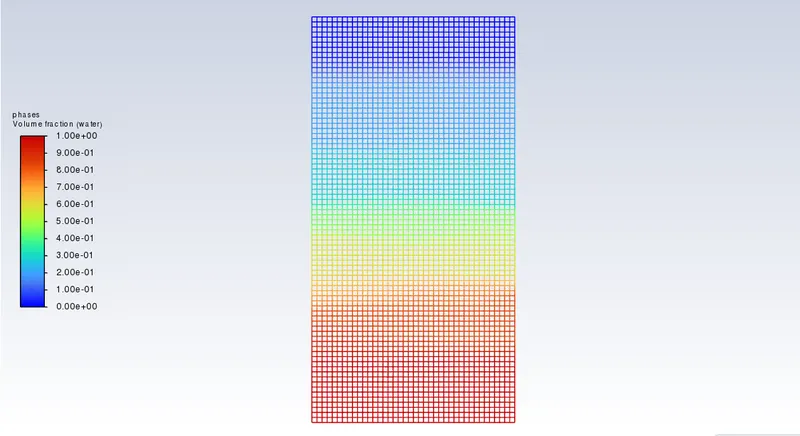
Volume Fraction:-

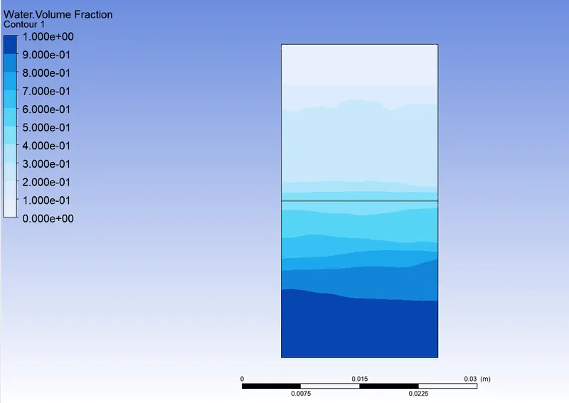
Solution Animation:-

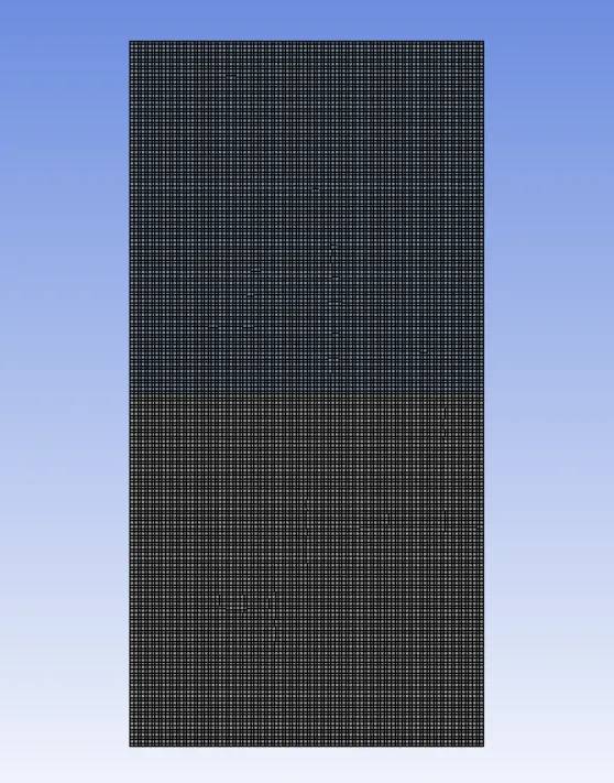
2. Mesh = 0.2 mm

Results:-

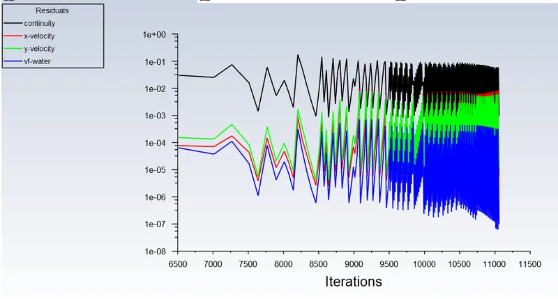
Residuals:-

Phases Contour:-

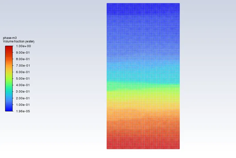
Volume Fraction:-

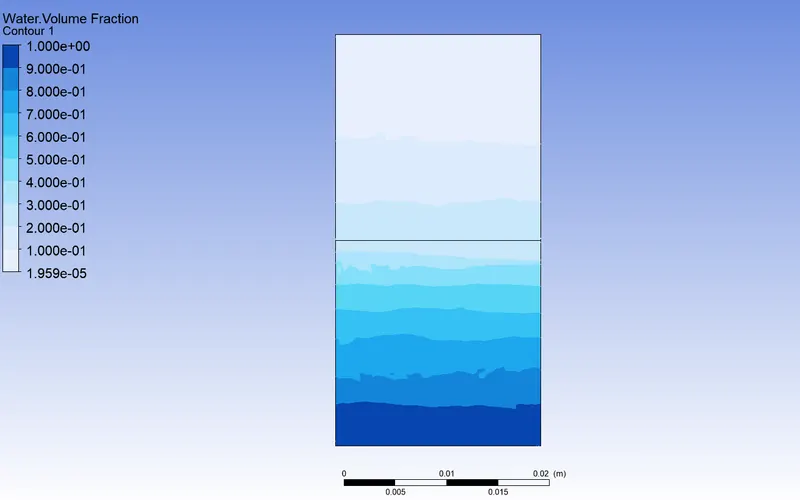
Solution Animation:-

Case 2:-

User-defined Material:

Density = 400 kg/m^3,

Viscosity = 0.001 kg/m-s

Mesh = 0.2 mm

Results:-

Residuals:-

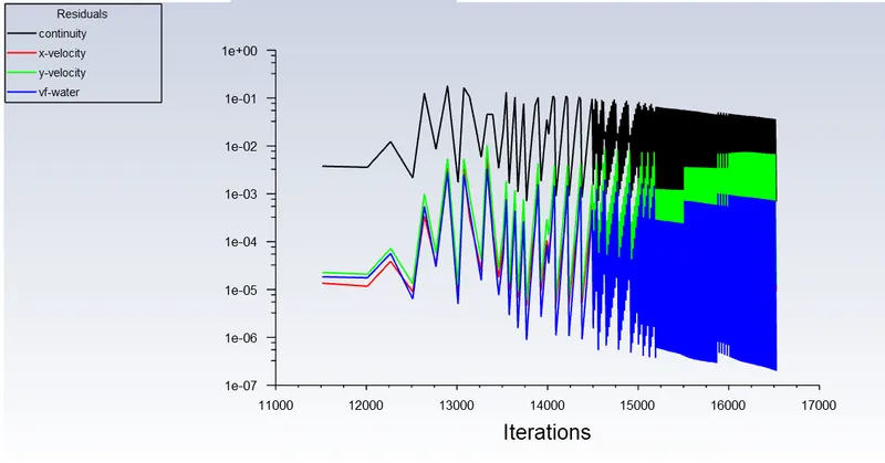
Phases Contour:-

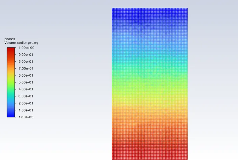
Volume Fraction:-

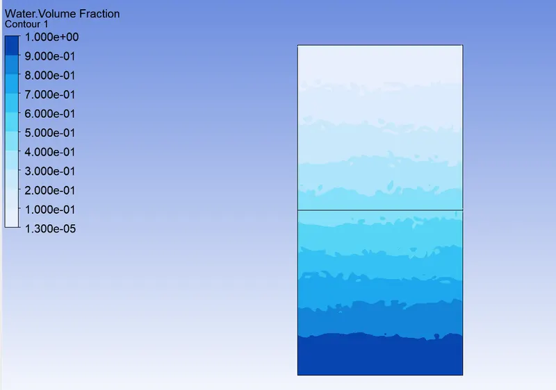
Solution Animation:-

why a steady-state approach might not be suitable for these types of simulations?

In this problem, we are observing the instabilities, when it is occurring. So we are not concerned about the final results, because the steady-state is more into capturing final results, but by transient approach, we can see the behavior of the solution and every instant such that capturing bubbles, Vortec, and shockwaves. Hence, the Transient approach is more suitable than the steady-state approach for this analysis.

Observation:-

It is observed that the more we refine the mesh, the more the simulation gets smoother about the variations that take place at the interface of the two fluids. As higher density fluid replaces lower density fluid, the formation of air bubbles and vortex take place which travels toward upward region with time. In case 2 We can observe more detailed results about the formation of waves and the initial formation of some air bubbles and later they travel upwards, generating shock waves. At the end of the simulation, we get two separated phases from each other.

Atwood Number:-

The Atwood number is dimensionless in fluid dynamics used in the study of harmonic instabilities in density stratified flows. it is a dimensionless density ratio:-

Atwood Number = `(rho1- rho2 ) / (rho1 + rho2)`

where,

= density of heavier fluid,

= density of lighter fluid,

Case 1:-

Heavier fluid (Water):-

Density (W):- 998.2 kg/m^3

Lighter fluid (Air):-

Density (A):- 1.225 kg/m^3

Atwood No. = [ Density(W) - Density (A)] / [ Density(W) + Density(A)]

Atwood No. = 0.996

Case 2:-

Heavier fluid (Water):-

Density (W):- 998.2 kg/m^3

Lighter fluid (Userdefined Material):-

Density (Userdefined Material):- 400 kg/m^3

Atwood No. = [ Density(W) - Density (A)] / [ Density(W) + Density(A)]

Atwood No. = 0.427

Atwood number is a crucial parameter in the study of Rayleigh–Taylor instability and Richtmyer–Meshkov instability. For the Atwood number close to 0, RT instability flows take from asymmetric "finger" of fluid; for Atwood no. close to 1, the much higher fluid "below" the heavier fluid takes the larger bubble-like plumps.