CFD analysis of Rayleigh Taylor Instability using VOF multiphase model
I. Aim: Numerical analysis and study of Rayleigh-Taylor instability in fluids.
II. Introduction:
The Rayleigh–Taylor instability, or RT instability (after Lord Rayleigh and G. I. Taylor), is the instability of an interface between two fluids of different densities which occurs when the lighter fluid is pushing the heavier fluid. Examples include the behavior of water suspended above oil in the gravity of Earth, mushroom clouds like those from volcanic eruptions and atmospheric nuclear explosions, supernova explosions in which expanding core gas is accelerated into denser shell gas, instabilities in plasma fusion reactors, and inertial confinement fusion.
As the RT instability develops, the initial perturbations progress from a linear growth phase into a non-linear growth phase, eventually developing "plumes" flowing upwards (in the gravitational buoyancy sense) and "spikes" falling downwards. In the linear phase, the fluid movement can be closely approximated by linear equations, and the amplitude of perturbations is growing exponentially with time. In the non-linear phase, perturbation amplitude is too large for a linear approximation, and non-linear equations are required to describe fluid motions. In general, the density disparity between the fluids determines the structure of the subsequent non-linear RT instability flows (assuming other variables such as surface tension and viscosity are negligible here).
Atwood Number:
The Atwood number (A) is a dimensionless number in fluid dynamics used in the study of hydrodynamic instabilities in density stratified flows. It is a dimensionless density ratio defined as:
`A = (rho_1-rho_2)/(rho_1+rho_2)`
where
- `rho_1` = density of heavier fluid
- `rho_2`= density of the lighter fluid
In Rayleigh–Taylor instability, the penetration distance of heavy fluid bubbles into the lighter fluid is a function of acceleration time scale-`Ag(t)^2`, where g is the gravitational acceleration and t is the time.
For A close to 0, RT instability flows take the form of symmetric "fingers" of fluid; for A close to 1, the much lighter fluid "below" the heavier fluid takes the form of larger bubble-like plumes.
CFD models based on mathematical analysis of Rayleigh Taylor waves:
1. Mass diffusion model: The mass diffusion equation describes the transport of mass and energy due to model viscosity and hence drives actual mixing in the fluids. Even if any configuration is Rayleigh-Taylor unstable, the diffusion process could be responsible for significant mixing if the viscosity is sufficiently large.
2. Multi-Fluid models: These models use a separate set of equations for each fluid in addition to the main flow equations and provide an accurate modeling framework for demixing by correctly capturing the relative motion of the different fluid fragments. The first step for the development of turbulence models is to perform Reynold averaging of the governing equations and resultant terms.
2.1. Two equation K-L turbulence model: The K-L turbulence model involves equations for turbulent kinetic energy K and turbulent length scale L. The starting point for deriving the model equations is the buoyancy-drag models for the self-similar growth of RT instabilities.
2.2. Three-equation K-L-a turbulence model: The three-equation model was developed as an extension to the two-equation K-L model by including a third equation for the turbulent mass-flux velocity.
2.3. Four-equation K-L-a-b turbulence model:
The four equation model was developed as an extension to the three-equation K-L model by including a fourth equation for density-specific volume covariance. The model can accurately reflect the effects of the changes in the density fluctuations.
3. Single fluid model:
3.1. Potential flow model: This model is valid for all instability changes from the linear stage through the early non-linear to the asymptotic but limited to Atwood number = 1. In this model, single-mode perturbation expands the flow equations to second-order around the bubble tips, hence obtaining an ordinary differential equation for the bubble velocity.
3.2. Buoyancy drag model: It is valid for every Atwood number but limited to the non-linear stages of the instability. It uses ordinary differential equations to evolve the width of the mixing layer. The bubble, or spike, amplitudes are described by balancing the inertia, buoyancy, and drag forces. These models cannot model multiple mixing interfaces; cannot be easily extended to 2 or 3 dimensions, and as a rule, do not address demixing, also known as counter gradient transport, i.e. reduction of total fluid masses within the mixing zone. To address the above problems, two-fluid(or multi-fluid)models have to be used.
3.3. Besnard-Harlow-Rauenzahn(BHR): It is a more advanced version of the single-fluid model. The BHR model is based upon the evolution equations arising from second-order correlations and gradient-diffusion approximations. Using a mass-weighted averaged decomposition, the original HR model includes full transport equations for the Reynold stresses, turbulent mass-flux velocity, density fluctuations, and the turbulent kinetic energy dissipation rate.
Rayleigh-Taylor instability Analysis:
In this project, 2D numerical Rayleigh-Taylor instability analysis of two fluids of different densities in a rectangular tank under the influence of gravity is carried in Ansys fluent software using the Volume of Fluid (VOF) multiphase model.
III Objectives:
- Perform the Rayleigh Taylor instability simulation for 2 different mesh sizes with the base mesh being 0.5 mm. Compare the results by showing the animations( Attach them via google drive). Observe the differences in the animation and explain the effect of mesh size on simulation. Also, explain why a steady-state approach might not be suitable for these types of simulation.[Choose Air and Water for this simulation]
- Run one more simulation with water and user-defined material(density = 400 kg/m3, viscosity = 0.001 kg/m-s) for refined mesh.
IV: Solving & Modelling approach:
2D CFD analysis is carried out in Ansys workbench using Fluent solver to simulate Rayleigh-Taylor instability using the Volume of Fluid (VOF) multiphase model. Three different cases were considered as follows:
Case1: Rayleigh-Taylor instability of Water-Air in a rectangular tank under the influence of gravity, with Water being on the top initially with a mesh element size of 5 mm.
Case2: Rayleigh-Taylor instability of Water-Air in a rectangular tank under the influence of gravity, with water being on the top initially for a case a refined mesh element size of 2 mm.
Case3: Rayleigh-Taylor instability of Water-UDM (user-defined material) in a rectangular tank with water being on the top initially under the influence of gravity , with a refined mesh element size of 2 mm.
V: Pre-processing and solver setting:
The first step in a CFD analysis is preprocessing. This includes preparing the geometry/ computational domain, discretization of the domain (meshing), assigning material properties, boundary conditions, solver setup.
1. Geometry/Domain:
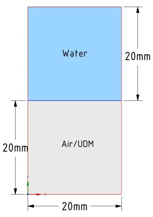
A 2D planar geometry of the rectangular tank is modeled in Spaceclaim. It is divided into two zones, one for lighter fluid (Air/UDM) and the other for water. The denser fluid zone is on the top initially. Further, share topology is enabled between the two zones to have conformal mesh. The following figure shows the geometry and zone details.
2. Domain discretization /Meshing:
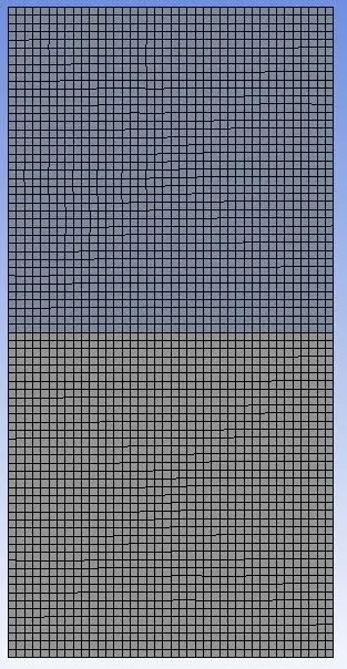
The 2D fluid zones are discretized into a finite number of control volumes using the Ansys meshing component. A 2D all hexahedral mesh is created. Two different mesh sizes are used:
Mesh-1: Element size of 5 mm is applied to all zones keeping all other settings to Ansys meshing defaults.
Mesh-2: Element size of 2 mm is applied to all zones keeping all other settings to Ansys meshing defaults.
 |
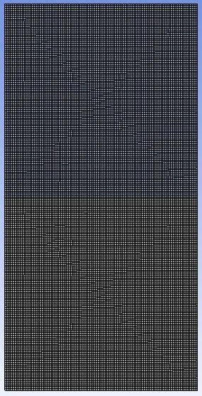 |
| Mesh-1 (Case1) | Mesh-2 (Case2/Case3) |
The generated 2D meshes have properties as follows:
| Mesh-1 | Mesh-2 | |
| Element Quality | 0.996 | 0.997 |
| Cell count | 3200 | 20000 |
| Min. Orthogonal Quality | 9.98963e-01 | 9.98194e-01 |
The properties of the fluids considered in this analysis are given below:
| Fluid | Density (kg/m^3) | Dynamic viscosity (kg/m-s) |
| Air at atmospheric conditions | 1.225 | 1.789E-5 |
| Water | 998.2 | 0.001003 |
| User-defined material (UDM) | 400 | 0.001 |
3. Solver setup:
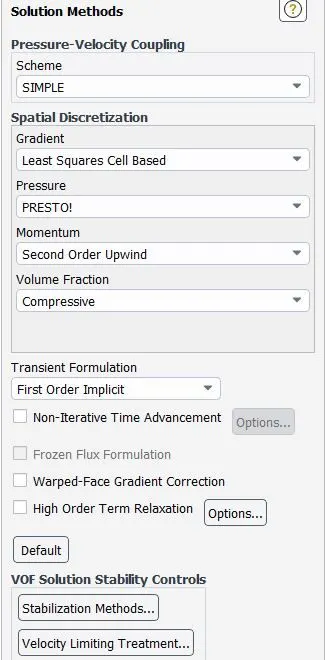
The 2D analysis is performed on the discretized domain(meshed model) in Ansys Fluent CFD software. A double-precision parallel solver with 4 cores is used. The double-precision solver uses 64-bit precision, which reduces the round-off error in the results. The solver setup details are given below:
| Solver type | Transient pressure-based solver |
| Gravity | -9.81 m/sec^2 (-ve Y direction) |
| Viscous model | Laminar |
| Multiphase model | Volume of fluid model (VOF) |
The Volume of Fluid (VOF) model is enabled to solve the interaction between the two different fluids of different densities under the influence of gravity. The VOF model parameters are as below:
| Volume fraction parameters | Implicit |
| Number of Eulerian phases | 2 |
| Primary phase | Air/UDM |
| Secondary phase | Water |
| Phase interaction | - |
IV Solution:
The solution is initialized with standard initialization. After this, the fluid zones have to be patched with the initial volume fraction of water. The details are as below:
| Top fluid zone | Bottom fluid zone | |
| Case1 | Water volume fraction = 1 | Water volume fraction = 0 (air) |
| Case2 | Water volume fraction = 1 | Water volume fraction = 0 (air) |
| Case3 | Water volume fraction = 1 | Water volume fraction = 0 (UDM) |
The solution is solved for 500 timesteps with a timestep size of 0.005 seconds. The Rayleigh-Taylor instability of the fluids is visualized by creating an animation of the water phase volume fraction over the solution process. The findings are discussed in the below section.
VI Results:
Case1: Rayleigh-Taylor instability between water-air with a mesh size of 0.5 mm
Initially, the water is at the top of the tank with air at the bottom. Due to the influence of gravity and density differences (Atwood number effects) Rayleigh-Taylor instabilities develop between the denser fluid water and lighter fluid air. This initiates large bubbles of air moving upward and water moving downward as shown in the below animation. After 500 timesteps with a timestep of 0.005 sec the water almost settles at the bottom of the tank. Increasing the number of timesteps, the final steady-state of water fully settling at the bottom can be visualized.
Case2: Rayleigh-Taylor instability between water-air with a mesh size of 0.2 mm
Initially, the water is at the top of the tank with air at the bottom. Due to the influence of gravity and density differences (Atwood number effects) Rayleigh-Taylor instabilities develop between the denser fluid water and lighter fluid air. This initiates large bubbles of air moving upward and water moving downward as shown in the below animation. Compared to Case1, the instabilities arise in this case with smaller bubbles size of air moving up. Also, the interaction between the two fluids is more pronounced with refined mesh size. This indicates that the Rayleigh-Taylor instability is sensitive to mesh size and having a refined mesh can accurately capture the physics of Rayleigh-Taylor instability.
Atwood number for Water-Air:
`A = (rho_1-rho_2)/(rho_1+rho_2)`
here `rho_1 = 998.2 (kg)/m^3`, density of water
`rho_2 = 1.225 (kg)/m^3`, density of Air
Therefore, `A = (998.2-1.225)/(998.2+1.225)`
`A = 0.9975 approx 1`
Since the Rayleigh-Taylor instabilities phenomenon is a transient process with instabilities occurring over a period of time based on the Atwood number, a steady-state approach is not feasible. A steady-state solution can only provide the equilibrium state achieved during a process. Hence, the steady-state approach is not feasible for studying Rayleigh-Taylor instabilities and a transient approach is required.
Case3: Rayleigh-Taylor instability between water-UDM with a mesh size of 0.2 mm
In this case, a user-defined material with density is higher than air considered with water for the refined mesh size. Since the UDM density is almost half of that of water, the instabilities arise very slowly at the Water-UDM with smaller finger-like structures and this initiates the instability causing the UDM to move upward and water moving downward as shown in the below animation. The settling time is more in this case due to the effect of a lesser density difference between the fluids.
Atwood number for Water-UDM:
`A = (rho_1-rho_2)/(rho_1+rho_2)`
here `rho_1 = 998.2 (kg)/m^3`, density of water
`rho_2 = 400 (kg)/m^3`, density of UDM
Therefore, `A = (998.2-400)/(998.2+400)`
A = 0.4275
| Atwood Number | |
| Water-Air | 0.9975 |
| Water-UDM | 0.4275 |
From the above table, it can be observed that the Atwood number for water-air is approximately equal to 1, which will give large plumes/bubbles of less dense fluid (air), during the Rayleigh-Taylor instability process as observed in the Case1 and Case2 animations above. The Atwood number for Water-UDM is 0.4275, which led to smaller finger-like instabilities of the less dense fluid (UDM) as observed in the Case3 animation above.
Conclusion:
The Rayleigh-Taylor instability is an instability mechanism occurring between fluids of different densities. The instability is dependent on the Atwood number. The objective of this project is to study the effect of mesh size and density of fluids on the Rayleigh-Taylor instability mechanism. Two different fluid combinations (Water-Air, Water-UDM) are considered with two mesh sizes. The refined mesh size cases have better interaction between the fluids during the instability process. For Water-Air, Atwood number is approximately equal to 1, which led to large plumes of air arising below the water. In the case of water-UDM, the Atwood number is around 0.428, which led to small finger-like (mushroom) shaped structures of less dense UDM fluid arising into the much higher dense fluid water.
References:
https://en.wikipedia.org/wiki/Atwood_number