Week 5 - Rayleigh Taylor Instability
Challange.
- What are some practical CFD models that have been based on the mathematical analysis of Rayleigh Taylor waves? In your own words, explain how these mathematical models have been adapted for CFD calculations.
- Perform the Rayleigh Taylor instability simulation for 2 different mesh sizes with the base mesh being 0.5 mm. Compare the results by showing the animations( Attach them from your google drive). Observe the differences in the animation and explain the effect of mesh size on simulation. Also, explain why a steady-state approach might not be suitable for these types of simulation.[ Choose Air and Water for this simulation]
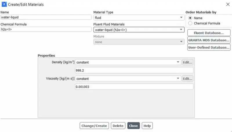
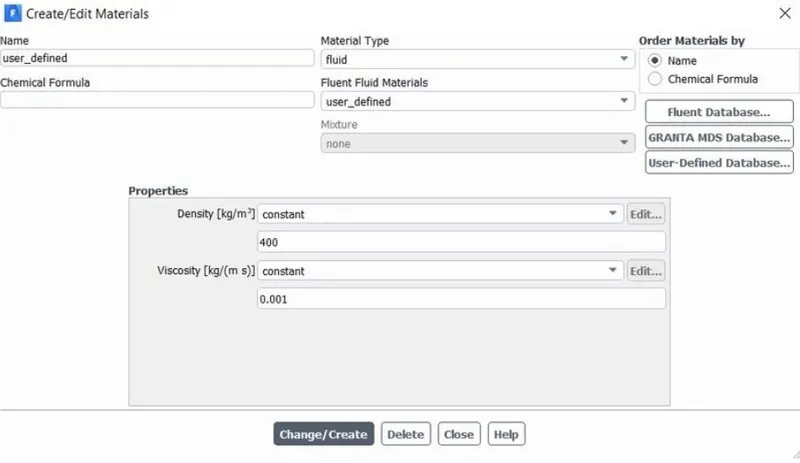
- Run one more simulation with water and user-defined material(density = 400 kg/m3, viscosity = 0.001 kg/m-s) for refined mesh.
- Define the Atwood Number. Find out the Atwood number for both the cases and explain how the variation in Atwood number in the above two cases affects the behavior of the instability.
Week 5 - Rayleigh Taylor Instability
Rayleigh Taylor Instability
The Rayleigh–Taylor instability, or RT instability, is the instability of an interface between two fluids of different densities which occurs when the lighter fluid is pushing the heavier fluid. Water suspended atop oil is an everyday example of Rayleigh–Taylor instability, and it may be modeled by two completely plane-parallel layers of immiscible fluid, the denser on top of the less dense one and both subject to the Earth's gravity. The equilibrium here is unstable to any perturbations or disturbances of the interface: if a parcel of heavier fluid is displaced downward with an equal volume of lighter fluid displaced upwards, the potential energy of the configuration is lower than the initial state. Thus the disturbance will grow and lead to a further release of potential energy, as the more dense material moves down under the (effective) gravitational field, and the less dense material is further displaced upwards. This was the set-up as studied by Lord Rayleigh. The important insight by G. I. Taylor was his realization that this situation is equivalent to the situation when the fluids are accelerated, with the less dense fluid accelerating into the more dense fluid. This occurs deep underwater on the surface of an expanding bubble and in a nuclear explosion.
As the RT instability develops, the initial perturbations progress from a linear growth phase into a non-linear growth phase, eventually developing "plumes" flowing upwards and "spikes" falling downwards. In the linear phase, the fluid movement can be closely approximated by linear equations, and the amplitude of perturbations is growing exponentially with time. In the non-linear phase, perturbation amplitude is too large for a linear approximation, and non-linear equations are required to describe fluid motions. In general, the density disparity between the fluids determines the structure of the subsequent non-linear RT instability flows. The difference in the fluid densities divided by their sum is defined as the Atwood number, A. For A close to 0, RT instability flows take the form of symmetric "fingers" of fluid; for A close to 1, the much lighter fluid "below" the heavier fluid takes the form of larger bubble-like plumes.
There are many CFD models which are based on Rayleigh-Taylor instability Richtmyer-Meshkov instabilities, Savart -Plateau-Rayleigh instability of water column, Iscous vortex single-mode bubble evolution model, Kelvin Helmholtz model etc.
Richtmyer - Meshkov instabilities -
It occurs when a shock wave interacts with an interface separating two fluids. It is adapted in monotone and implicit large eddy-simulations, large eddy simulation, and Navier-stroke simulations. A multicomponent form of dissipative compressible fluid dynamics equation was solved to simulate the interaction of shock wave with a box of SF6. central difference methods were evolved to adaptive grid large-eddy simulations of the Richtmyer-Meshkov instability.
Savart -Plateau-Rayleigh instability of water column -
Felix Savart proposed a study of the shape of a liquid stream. In letting a jet on a solid disk, the mass and momentum of the incident jet are radially distributed, symmetrically. The expansion is bounded to a radial location after it breaks into the ligament and drops. This is the Savart instability. This is adapted in CFD to simulate liquid jet imping.
Bubble evolution model -
it is an extension of the inviscid model. In it, RTI has divided into two phases initial vortex and diffusion process at the interface of two fluids. This model is used to predict earlier stages of RTI for low Atwood number.
Kelvin-Helmholtz instability -
It is a hydrodynamic instability in which where there is density and velocity differences in the fluids are continuous. For the Kelvin-Helmholtz instability, small perturbations of the shear layer trigger its evolution into an array of large-scale vortices dissipating into smaller ones. This instability model is used to simulate climate dynamics, two immiscible fluids moving co-currently, modeling the dynamics of jet, etc.
- Procedure-
Geometry
|
|
|
|
|
|
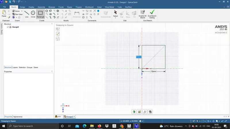
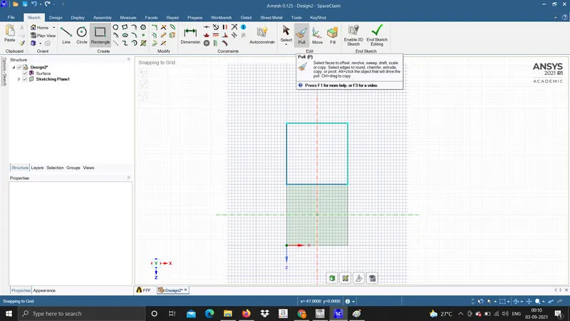
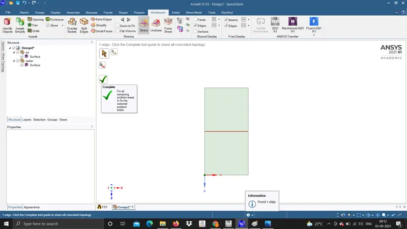
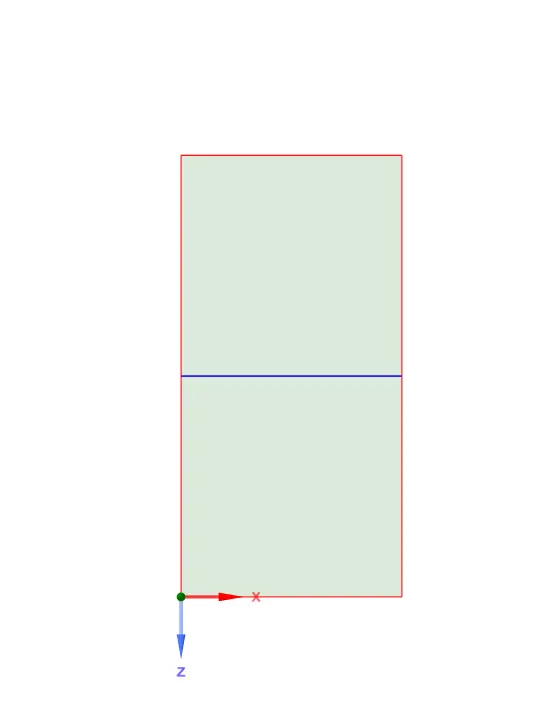
Final Geometry
- MESHING
| Case 1 | 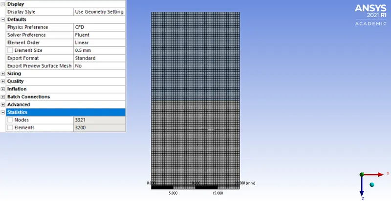 |
| Case 2 | 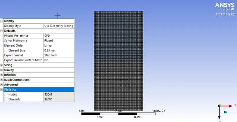 |
| Case 3 | 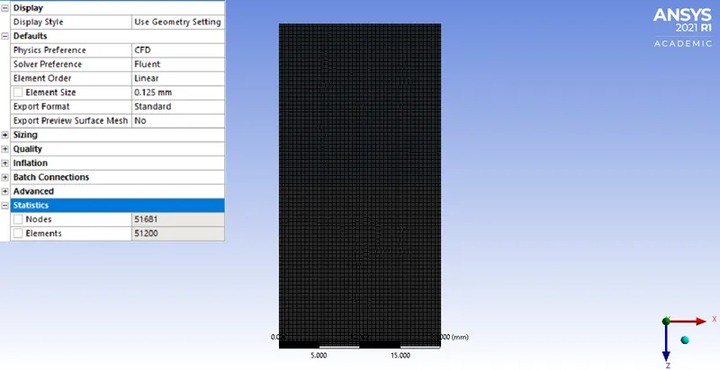 |
- SETUP
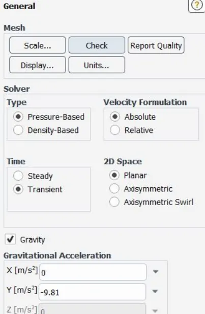
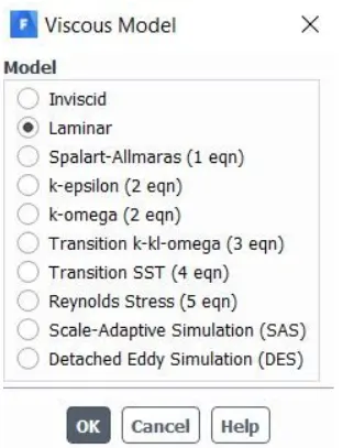
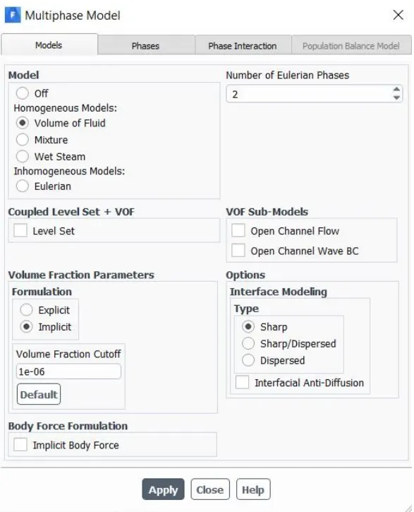
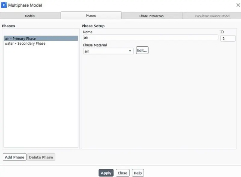
PHYSICS
|
 |
|
 |
|
 |
|
 |
|
 |
|
 |
|
 |
|
 |
|
 |
- RESULTS
- CASE 1
- SCALAR RESIDUALS
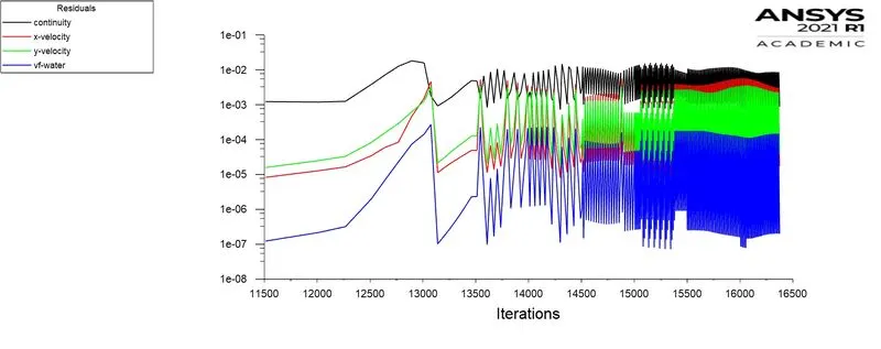
- CASE 2
- SCALAR RESIDUALS
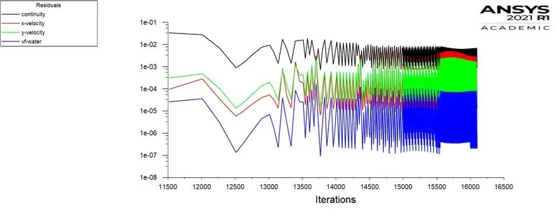
- CASE 3
- SCALAR RESIDUALS
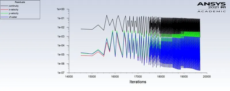
- USER-DEFINED MATERIAL
- SCALAR RESIDUALS
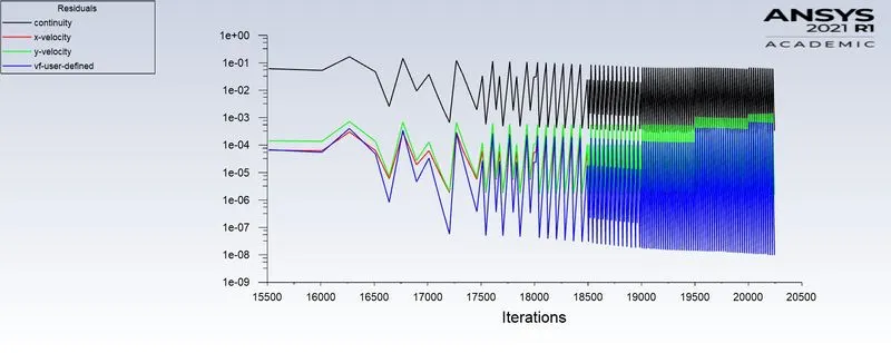
Atwood Number
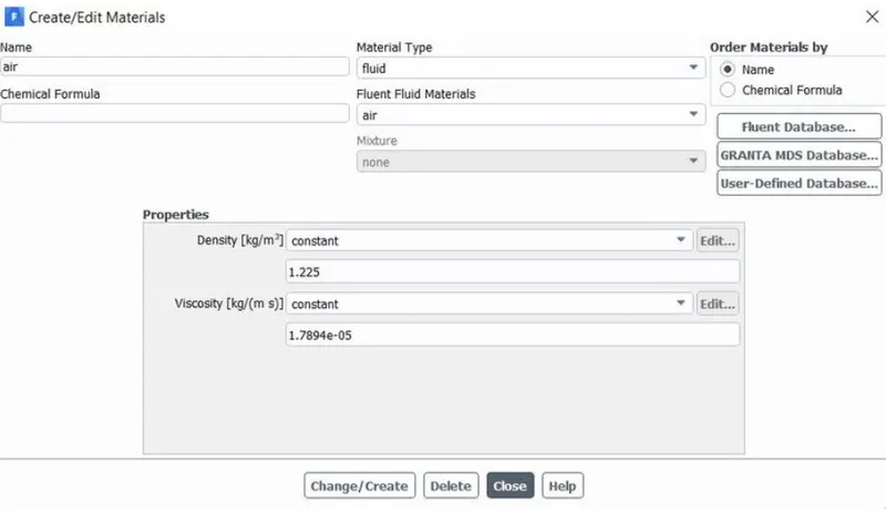
It is diamentionless density ratio, atwood number is the number to study hydrodynamic instabilities in density stratified flow.
`A=(rho_1-rho_2)/(rho_1+rho_2)`
where,
`rho_1` = density of heavier fluid
`rho_2`=density of lighter fluid
| Case 1- For air and water | Case 1- For air and user-defined |
|
`rho_1` = 998.2 kg/m^3 `rho_2`= 1.225 kg/m^3 |
`rho_1` = 998.2 kg/m^3 `rho_2`= 400 kg/m^3 |
| `A=(998.2-1.225)/(998.2+1.225)` | `A=(998.2-400)/(998.2+400)` |
| A= 0.9975 | A = 0.427 |
- For the case of smaller Atwood Number, the density difference between the two sides of the interface is small so the density distribution of the upper and lower layers is symmetrical.
- It is found that the initial density stratification caused by compressibility plays a stabilizing role, while the expansion-compression effect of flow plays a destabilizing role.
- For higher Atwood number influence of initial stratification decreases and instability caused by expansion compression effect increases.
- CONCLUSION
- In this challenge, the simulation starts with the state of hydrostatic equilibrium, and the Rayleigh Taylor instability is observed at the interference when a lower density fluid pushes a higher density fluid due to which formation of shock waves at the interface takes place.
- Formation of air bubbles starts taking place, which compresses the heavy fluid around it, due to which shock waves of multidimensional fashion generates and it gets more stronger as it moves upward.
- It is observed that the more we refine the mesh, the more the simulation results get smoother about the irregularities that take place at the interface of the two fluids.
- As higher density fluid replaces lower density fluid, the formation of air bubbles and vortex takes place, which travels towards the upward region with time.
- In case-3, we can see the more detail results about the formation of waves and the formation of some air bubbles that get trapped at the lower region during the initial stage and then they travel towards the upper region, generating shock waves.
- At the end of the simulation, it is to be observed that the two phases get separated from each other though, we can see some diffusivity between them which is a volume fraction of air and water.
- In the Rayleigh- Taylor Instability, due to a sudden collapse in the layer between the denser and lighter fluid spike generation takes place which is obviously time dependent, hence using a steady state solver will not work as we are interested in the flow parameters with respect to time.