Week 5.1 - Mid term project - Solving the steady and unsteady 2D heat conduction problem
Mid term project - Solving the steady and unsteady 2D heat conduction problem
- THEORY : In conduction, the heat flow is within and through the body itself. In contrast, in heat transfer by thermal radiation the transfer is often between bodies, which may be separated spatially. Also possible is the transfer of heat by a combination of conduction and thermal radiation. In convection, the internal energy is carried between bodies by a moving material carrier. In gases and liquids, conduction is due to the collisions and diffusion of molecules during their random motion.
- Eqation of heat in 3D general case.
`(delu)/(delt)= K.((del^2u)/(delx^2)+(del^2u)/(dely^2)+(del^2u)/(delz^2))`
where K = coefficient of diffusivity
TYPES OF HEAT CONDUCTION
- Steady-state Conduction
Steady-state conduction is the form of conduction that happens when the temperature diffrences driving the conduction and constant, so that the spatial distributionof tempreture the conducting object does not change any further
HEAT CONDUCTION IN STEADY STATE 2-DIMENSION
`(T_l-2*T_p+T_r)/(delx^2)+(T_t-2*T_p+T_b)/(dely^2)=0 ...........(1)`
The spacing in x & y direction can be defined as dx, dy respectively. Here is the derivation for descretisation, which could be used in program.
For SOR method it turns out to be a small changr with the intoduction of the relaxation factor.
`(T_ij)^(k+1)=(T_ij)^(k)*(1-omega)+omega*T_gs(i,j)`
eq 1 can be simplified as follows
`2*((T_p)/(delx^2)+T_p/(dely^2))=(T_l+T_r)/(delx^2)+(T_t+T_b)/(dely^2)`
`T_p( 2*(T_p)/(delx^2)+T_p/(dely^2))=RHS`
`K=2[(delx^2+dely^2)/(delx^2*dely^2)] ....(2)`
Let us now solve the programe using eq. 2
so the equation for tempreature field will be
`T_(i,j)=1/K*((T_(i-1,j)+T_(i+1,j))/(Deltax^2)+(T_(i,j-1)+T_(i,j+1))/(Deltay^2))`
code for jacobi iterations
#code foe 2d temprature distribution at steady state
clear all
close all
clc
%steady flow heat conduction
%inputs

nx=11;
ny=11;

%to calculate the values of x &y
x= linspace(0,1,nx);
y= linspace(0,1,ny);

dx=x(2)-x(1);
dy=dx;

%assignin BC

Temp_left=400;
Temp_top=600;
Temp_right=800;
Temp_bottom=900;

T= 300*ones(nx,ny);

T(2:ny-1,1)=Temp_left;
T(2:ny-1,nx)=Temp_right;
T(1,2:nx-1)=Temp_top;
T(ny,2:nx-1)=Temp_bottom;

T(1,1)= (Temp_top+Temp_left)/2;
T(nx,ny)= (Temp_right+Temp_bottom)/2;
T(1,ny)= (Temp_top+Temp_right)/2;
T(nx,1)= (Temp_left+Temp_bottom)/2;

k=2*(1/(dx^2)+1/(dy^2));

T_initial=T;
Told=T;

iterative_solver=1;
error=9e9;
tol=1e-4;

%jacobi method
if iterative_solver == 1
jacobi_iter=1;
  while(error>tol)
    for i= 2:nx-1
        for j= 2:ny-1

        T(i,j)=(1/k)*((Told(i-1,j)+Told(i+1,j))/(dx^2)+(Told(i,j-1)+Told(i,j+1))/(dy^2));

         end
        end
        error =max(max(abs(Told-T)));
        Told =T;
        jacobi_iter=jacobi_iter+1;
end
figure(1)
contour(x,y,T)
clabel(contourf(x,y,T))
colorbar
colormap
colormap(jet)
set(gca,'ydir','reverse')
xlabel('X axis')
ylabel('y axis')
title(sprintf('Jacobi method teration number =%d',jacobi_iter));
pause(0.03)
end
PLOT FOR JACOBI METHOD
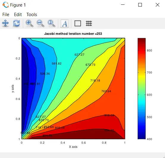
- NUMBER OF ITERATIONS- 253
CODE FOR GS METHOD
#code foe 2d temprature distribution at steady state
clear all
close all
clc
%steady flow heat conduction
%inputs

nx=11;
ny=11;

%to calculate the values of x &y
x= linspace(0,1,nx);
y= linspace(0,1,ny);

dx=x(2)-x(1);
dy=dx;
error= 9e9;
tol=1e-4;

%assignin BC

Temp_left=400;
Temp_top=600;
Temp_right=800;
Temp_bottom=900;

T= 300*ones(nx,ny);

T(2:ny-1,1)=Temp_left;
T(2:ny-1,nx)=Temp_right;
T(1,2:nx-1)=Temp_top;
T(ny,2:nx-1)=Temp_bottom;

T(1,1)= (Temp_top+Temp_left)/2;
T(nx,ny)= (Temp_right+Temp_bottom)/2;
T(1,ny)= (Temp_top+Temp_right)/2;
T(nx,1)= (Temp_left+Temp_bottom)/2;

T_initial=T;
Told=T;

iterative_solver=2;
k=2*(1/(dx^2)+1/(dy^2));

%gs method
if iterative_solver == 2
gs_iter=1;
  while(error>tol)
    for i= 2:nx-1
        for j= 2:ny-1

        T(i,j)= 1/k*((Told(i-1,j)+Told(i+1,j))/(dx^2)+(T(i,j-1)+Told(i,j+1))/(dy^2));

         end
        end
        error =max(max(abs(Told-T)));
        Told =T;
        gs_iter=gs_iter+1;
end
figure(1)
contour(x,y,T)
clabel(contourf(x,y,T))
colorbar
colormap
colormap(jet)
set(gca,'ydir','reverse')
xlabel('X axis')
ylabel('y axis')
title(sprintf('gs method teration number =%d',gs_iter));
pause(0.03)
end
PLOT FOR GS METHOD
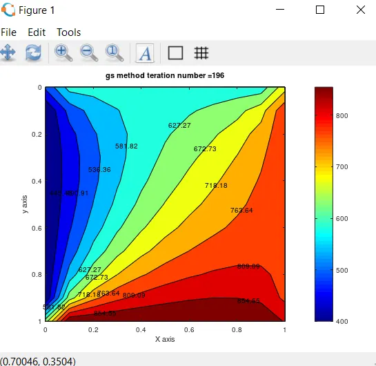
- NUMBER OF ITERATIONS- 136
CODE FOR SOR METHOD
#code foe 2d temprature distribution at steady state
clear all
close all
clc
%steady flow heat conduction
%inputs

nx=11;
ny=11;

%to calculate the values of x &y
x= linspace(0,1,nx);
y= linspace(0,1,ny);

dx=x(2)-x(1);
dy=dx;
error= 9e9;
tol=1e-4;
omega=1.2;

%assignin BC

Temp_left=400;
Temp_top=600;
Temp_right=800;
Temp_bottom=900;

T= 300*ones(nx,ny);

T(2:ny-1,1)=Temp_left;
T(2:ny-1,nx)=Temp_right;
T(1,2:nx-1)=Temp_top;
T(ny,2:nx-1)=Temp_bottom;

T(1,1)= (Temp_top+Temp_left)/2;
T(nx,ny)= (Temp_right+Temp_bottom)/2;
T(1,ny)= (Temp_top+Temp_right)/2;
T(nx,1)= (Temp_left+Temp_bottom)/2;

T_initial=T;
Told=T;

iterative_solver=2;
k=2*(1/(dx^2)+1/(dy^2));

%sor method
if iterative_solver == 2
sor_iter=1;
  while(error>tol)
    for i= 2:nx-1
        for j= 2:ny-1

        T(i,j)= omega*(1/k*((T(i-1,j)+Told(i+1,j))/(dx^2)+(T(i,j-1)+Told(i,j+1))/(dy^2)))+(1-omega)*Told(i,j);

         end
        end
        error =max(max(abs(Told-T)));
        Told =T;
        sor_iter=sor_iter+1;
end
figure(1)
contour(x,y,T)
clabel(contourf(x,y,T))
colorbar
colormap
colormap(jet)
set(gca,'ydir','reverse')
xlabel('X axis')
ylabel('y axis')
title(sprintf('sor method teration number =%d',sor_iter));
pause(0.03)
end
PLOT FOR SOR METHOD
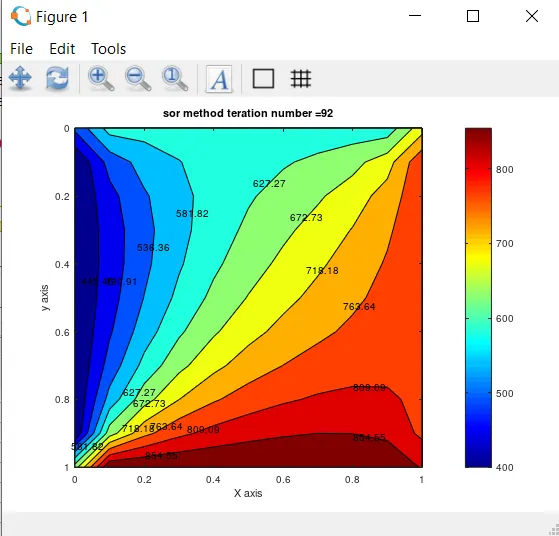
- NUMBER OF ITERATIONS- 92
- CONCLUSION-
- The number of iterations of jacobi, GS and SOR is 253, 136 and 92 respectively.
- The convergence rate is faster in all the three method in the steady state.
- In steadt state numbers of iterations in Jacobi method is greater then GS method and SOR method
- And number of iterations in SOR method is lesser then GS and Jacobi method.
- Therefore, the convergencen rate of SOR is faster then Jacobi and GS method.
- Trensient conduction
During any period in which temperatures changes in time at any olace within an object, the mode of thermal energy flow is termed trensient conduction.
If the temperature of the body varies at any point with time as well as position then its the transient heat conduction.
The 2D formula for heat conduction can be given as follows:
`(delT)/(delt)= alpha*((del^2T)/(delx^2)+(del^2T)/(dely^2))`
`(T_p^(n+1)-T_p^(n))/(delt)= alpha*((T_l-2*T_P+T_r)/(delx^2) +(T_t-2*T_P+T_b)/(dely^2) )^(n or n+1)`
`k1= alpha*((delt)/(delx^2))`
`k2= alpha*((delt)/(dely^2))`
here n is for explicite method and n+1 for implicit method
The final equation would be
- For explicite
-
`T_p^(n+1) =T_p^(n)+k1*(T_l-2*T_p+T_r)^(n)+k2*(T_t-2*T_p+T_b)^(n)`
- For implicite
`T_p^(n+1) =1/(1+2k1+2*k2)*(T_p^(n)+k1*(T_l+T_r)^(n+1)+k2*(T_t+T_b)^(n))`
- TRANSIENT ANALYSIS BY EXPLICIT METHOD
#code foe 2d temprature distribution at steady state
clear all
close all
clc
%steady flow heat conduction
%inputs

nx=10;
ny=10;
nt=1400;

%to calculate the values of x &y
x= linspace(0,1,nx);
y= linspace(0,1,ny);

dx=x(2)-x(1);
dy=dx;
error= 9e9;
tol=1e-4;
dt=1e-3;

%assignin BC

Temp_left=400;
Temp_top=600;
Temp_right=800;
Temp_bottom=900;

T= 300*ones(nx,ny);

T(2:ny-1,1)=Temp_left;
T(2:ny-1,nx)=Temp_right;
T(1,2:nx-1)=Temp_top;
T(ny,2:nx-1)=Temp_bottom;

T(1,1)= (Temp_top+Temp_left)/2;
T(nx,ny)= (Temp_right+Temp_bottom)/2;
T(1,ny)= (Temp_top+Temp_right)/2;
T(nx,1)= (Temp_left+Temp_bottom)/2;

T_initial=T;
Told=T;

iterative_solver=1;
alpha=1.4;
k1=alpha*(dt/(dx^2));
k2=alpha*(dt/(dy^2));

%explicite method

explicite_iter=1;

for k=1:nt
  error=9e9;
  while(error>tol)
    for i= 2:nx-1
        for j= 2:ny-1
       term1=Told(i,j);
       term2=k1*(Told(i+1,j)-2*Told(i,j)+Told(i-1,j));
       term3=k2*(Told(i,j+1)-2*Told(i,j)+Told(i,j-1));

       T(i,j)= term1+term2+term3;
         end
        end
        error =max(max(abs(Told-T)));
        Told =T;
        explicite_iter=explicite_iter+1;
end
  T_initial=T;
end
figure(1)
contour(x,y,T)
clabel(contourf(x,y,T))
colorbar
colormap
colormap(jet)
set(gca,'ydir','reverse')
xlabel('X axis')
ylabel('y axis')
title(sprintf('explicite method teration number =%d',explicite_iter));
pause(0.00000000000003)
PLOT
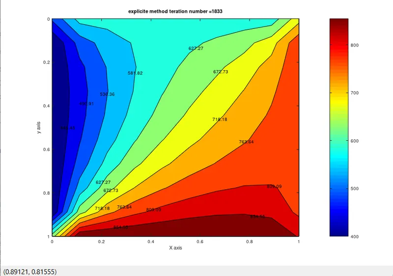
- NUMBER OF ITREATIONS- 1833
To solve the implicit method by jacobi GS and SOR method the above formula is simulated in the programe
Three method are as follow
- JACOBI METHOD
#code for 2d temprature distribution at transient state
clear all
close all
clc
%inputs

nx=10;
ny=10;
nt=1400;

%to calculate the values of x &y
x= linspace(0,1,nx);
y= linspace(0,1,ny);

dx=x(2)-x(1);
dy=dx;
error= 9e9;
tol=1e-4;
dt=1e-3;

%assignin BC

Temp_left=400;
Temp_top=600;
Temp_right=800;
Temp_bottom=900;

T= 300*ones(nx,ny);

T(2:ny-1,1)=Temp_left;
T(2:ny-1,nx)=Temp_right;
T(1,2:nx-1)=Temp_top;
T(ny,2:nx-1)=Temp_bottom;

T(1,1)= (Temp_top+Temp_left)/2;
T(nx,ny)= (Temp_right+Temp_bottom)/2;
T(1,ny)= (Temp_top+Temp_right)/2;
T(nx,1)= (Temp_left+Temp_bottom)/2;

T_initial=T;
Told=T;

iterative_solver=1;
alpha=1.4;
k1=alpha*(dt/(dx^2));
k2=alpha*(dt/(dy^2));

%jacobi method

jacobi_iter=1;

for k=1:nt
  error=9e9;
  while(error>tol)
    for i= 2:nx-1
        for j= 2:ny-1
       term1=1/(1+(2*k1)+(2*k2));
       term2=k1*term1;
       term3=k2*term1;
       H= Told(i-1,j)+Told(i+1,j);
       V=Told(i,j+1)+Told(i,j-1);
       T(i,j)= T_initial(i,j)*term1+H*term2+V*term3;
         end
        end
        error =max(max(abs(Told-T)));
        Told =T;
        jacobi_iter=jacobi_iter+1;
end
  T_initial=T;

figure(1)
contour(x,y,T)
clabel(contourf(x,y,T))
colorbar
colormap
colormap(jet)
set(gca,'ydir','reverse')
xlabel('X axis')
ylabel('y axis')
title(sprintf('jacobi method iteration number =%d',jacobi_iter));
pause(0.00000000000003)
end- PLOT
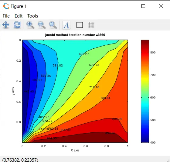
- NUMBER OF ITERATIONS - 3666
- GS METHOD
#code foe 2d temprature distribution at TRANSIENT state
clear all
close all
clc

%inputs

nx=10;
ny=10;
nt=1400;

%to calculate the values of x &y
x= linspace(0,1,nx);
y= linspace(0,1,ny);

dx=x(2)-x(1);
dy=dx;
error= 9e9;
tol=1e-4;
dt=1e-3;

%assignin BC

Temp_left=400;
Temp_top=600;
Temp_right=800;
Temp_bottom=900;

T= 300*ones(nx,ny);

T(2:ny-1,1)=Temp_left;
T(2:ny-1,nx)=Temp_right;
T(1,2:nx-1)=Temp_top;
T(ny,2:nx-1)=Temp_bottom;

T(1,1)= (Temp_top+Temp_left)/2;
T(nx,ny)= (Temp_right+Temp_bottom)/2;
T(1,ny)= (Temp_top+Temp_right)/2;
T(nx,1)= (Temp_left+Temp_bottom)/2;

T_initial=T;
Told=T;

iterative_solver=1;
alpha=1.4;
k1=alpha*(dt/(dx^2));
k2=alpha*(dt/(dy^2));

%gs method

gs_iter=1;

for k=1:nt
  error=9e9;
  while(error>tol)
    for i= 2:nx-1
        for j= 2:ny-1
       term1=1/(1+(2*k1)+(2*k2));
       term2=k1*term1;
       term3=k2*term1;
       H= T(i-1,j)+Told(i+1,j);
       V=T(i,j+1)+Told(i,j-1);
       T(i,j)= T_initial(i,j)*term1+H*term2+V*term3;
         end
        end
        error =max(max(abs(Told-T)));
        Told =T;
        gs_iter=gs_iter+1;
end
  T_initial=T;

figure(1)
contour(x,y,T)
clabel(contourf(x,y,T))
colorbar
colormap
colormap(jet)
set(gca,'ydir','reverse')
xlabel('X axis')
ylabel('y axis')
title(sprintf('gs method iteration number =%d',gs_iter));
pause(0.00000000000003)
end- PLOT
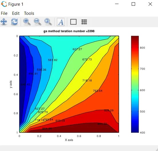
- NUMBER OF ITERATIONS-3398
- SOR METHOD
#code foe 2d temprature distribution at TRANSIENT state
clear all
close all
clc

%inputs

nx=11;
ny=11;
nt=1400;

%to calculate the values of x &y
x= linspace(0,1,nx);
y= linspace(0,1,ny);

dx=x(2)-x(1);
dy=dx;
error= 9e9;
tol=1e-4;
dt=1e-3;
omega=1.1;

%assignin BC

Temp_left=400;
Temp_top=600;
Temp_right=800;
Temp_bottom=900;

T= 300*ones(nx,ny);

T(2:ny-1,1)=Temp_left;
T(2:ny-1,nx)=Temp_right;
T(1,2:nx-1)=Temp_top;
T(ny,2:nx-1)=Temp_bottom;

T(1,1)= (Temp_top+Temp_left)/2;
T(nx,ny)= (Temp_right+Temp_bottom)/2;
T(1,ny)= (Temp_top+Temp_right)/2;
T(nx,1)= (Temp_left+Temp_bottom)/2;

T_initial=T;
Told=T;
T_end=T;

iterative_solver=1;
alpha=1.4;
k1=alpha*(dt/(dx^2));
k2=alpha*(dt/(dy^2));

%sor method

sor_iter=1;

for k=1:nt
  error=9e9;
  while(error>tol)
    for i= 2:nx-1
        for j= 2:ny-1
       term1=1/(1+(2*k1)+(2*k2));
       term2=k1*term1;
       term3=k2*term1;
       H= T(i-1,j)+Told(i+1,j);
       V=T(i,j+1)+Told(i,j-1);
       T(i,j)= T_initial(i,j)*term1+H*term2+V*term3;
       T_end(i,j)=((1-omega)*Told(i,j)+(T(i,j)*omega));
         end
        end
        error =max(max(abs(Told-T)));
        Told =T_end;
        sor_iter=sor_iter+1;
end
  T_initial=T_end;

figure(1)
contour(x,y,T)
clabel(contourf(x,y,T))
colorbar
colormap
colormap(jet)
set(gca,'ydir','reverse')
xlabel('X axis')
ylabel('y axis')
title(sprintf('sor method iteration number =%d',sor_iter));
pause(0.00000000000003)
end- PLOT
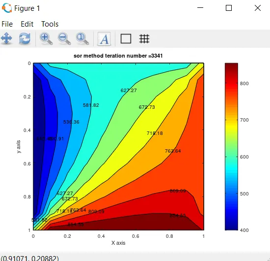
- NUMBER OF ITERATIONS- 3341
- CONCLUSION
- As the method changes the number of iteration changes with each method.
- The number of iteration in jacobi is 3666 , in GS 3398 method and in SOR it's 3341.
- Iterations in SOR is lesser then Jacobi and GS method, ie it computes faster then the Jacobi and SOR.
- So from these we could say SOR method is the best for solving implicit equations.