Week 9 - FVM Literature Review

FVM Literature Review

FINITE VOLUME METHOD

1. Finite volume method is a method which represent and evaluates partial diffrential equation in the form of algebric equations.
2. The basic laws of fluid dynamics are conservation laws that states and express the conservation of mass,conservation of momentum & conservation of energy in the volume closed by a surface.
3. in finite volume method volume integrate in PDE that contains a divergence term are converted.
4. These terms are evaluated as flux at the surface of each finite volume.
5. because the flux entering a given volume is identical to that the leaving the addjecent tvolume, these method are conservative.
6. Another advantage of the finite volume method is that it is easily formulated to allow for unstructured meshes.
7. This elements of the mesh is called as control volumes, the integration of partial diffrential equation over each control volume results in a balanced equation.
8. Finete volume refers to the small volume sourounding each node point on a mesh.
9. In FVM equation are written in a entire volume and no assumptions were made over the shape of the volume.
10. Inside tthis particular volume, all the flow quantites are conserved.

Differences between FDM & FVM

Finite diffrence method-

• FDM method is the numerical method which uses Partial Diffrence Equations.
• Finite difference method is created from basic defination of differentiation that is `(df)/dx =(f(x+h)-f(x))/h`
• Mapping in a governingb equation is difficult and FDM impliments complex mapping where needed.
• Method is easy but not reliable forn conventional diffrential equations and solutions having shocks.
• Exteneding to higher order accuracy is very simple.
• In FDM discretizartion is based upon the diffrential form of the PDE to be solved. Each derivative is replaced with an approximate difference formula. The computational domain is usually divided into hexahral cells, and the solution will be obtained at each nodal point.
• Finite diffrence method uses regular grid.
• FDM is easiest to understand and when the physical grid is cartesian. we cannot implement this method, when the grid are not aligned along x, y or z directions.
• Incremental time step need to be smaller then the critical value for stability.
• The discretizwation results in a system of equation of the variables at nodal points, and once a solution is found, then we have a discrete representation of the solution.

Finite Volume method-

• It is a numerical tool that is borrowed from calculus of variation. Here we assume some trial function and multiply that trial function with weighting function.
• Then this weighting function is multiplied with trial function then integrated over the control volume (weak from) and equated to zero(This procedure will differ for different types of FEM but theme is same).Then we get one set of algebraic equations. Solvingthat will give solution.
• Here we are working only in error and differential equation some times conservative law may be violated. This method is more accurate than PDEs.
• Here higher order accuracy is achieved by using higher order basis file) shape functions. Extending to higher order accurate calculations are expensive in computation and Mathematical formulation especially for non-linear PDEs.
• Mostly suitable for Heat transfer, Structural mechanics, vibrational analysis etc,
• The PDE is written in a form which can be solved for a given finite volume for cell). The computational domain is discretized into finite volume and then for every volume the governing equation is solved.
• The resulting system of equation usually involves fluxes of the conserved variable, and thus the calculation of fluxes is very important in FVM.
• The basic advantage is it dose not require the use of structured grid, and the effort to convert the given mesh into structured numerical grid internally is completely avoided
• As with FDM, the resulting approximate solution is a discrete, but the variables are typically placed at cell centers rather than at nodal points.
• This is not always true. As there are also face-centered finite volume methods. In any case, the values of field variables at non storage ocations are obtained using interpolation.

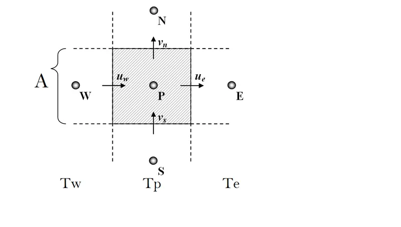
• The governing equations are calid at every point in the fomain which means it is valid in the entires control volume.

• now multiply the governing equation with dv and integrate it.

`int(del/(delx) (alpha (delT)/(delx) )+s)dv =0`

`int(del/(delx) (alpha (delT)/(delx) ))dv+int(s)dv =0`

where `dv=A*dv`

`int_w^e(del/(delx) (alpha (delT)/(delx) ))Adv+int(s)dv =0`

`[alphaA ((delT)/(delx) )]_w^e + dots dv=0`

Where `dot s` is the avrage of source term

`[alphaA ((delT)/(delx_e) )] -[alphaA ((delT)/(delx_W) )] + dots dv=0`

The above equation states

Heat flux out - heat flux in + `s_u +s_pT_p`

`alphaA [(T_e-T_p)/(Deltax) ]-alphaA [(T_p-T_w)/(Deltax) ]+ dots dv=0`