Week 7 - Simulation of a 1D Super-sonic nozzle flow simulation using Macormack Method

Simulation of a 1D Super-sonic nozzle flow simulation using Macormack Method

NOZZLE:-

A nozzle is a device designed to controled the direction or charachteristics of a fluid flow as it exits an enclosed chamber or pipe. A nozzle is often a pipe or tube of varyingn cross section area, and it can be used to direct or modify the flow of a fluid.

Nozzle are usualy used to control the rate of flow, speed, direction, mass, shape, and the pressure of the stream that emerges from them.

There are three major types of nozzle

1. Convergent nozzle
2. Divergent nozzle
3. COnvergent-divergent nozzle

For the week course a understanding a convergent-divergent nozzle and lets perform.

CONVERGENT-DIVERGENT NOZZLE

The Nozzle is used to obtain a supersonic stream staerting feom low speed at the inlet. Then the Mach number should increase from Ma=0 near the inlet to Ma>1 at the exit. It is clear that the nozzle must converge in the subsonic portion and diverge in the supersom=nic portion. Such a nozzle is called a Convergent-divergent nozzle.

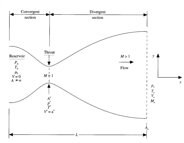
We consider the steady, isentropic flow through a convergent-divergent nozzle as given below. The flow at the Nozzle comes from the reservior where the oressure and temprature are denoted by `P_0` &`T_0`. The cross-section area of the reservior is large `(A=oo)`, and hence the velocity is very small `(V=0)`. Thus `P_0` &`T_0` are the stagnation values, or total pressure and total temperature, respectively. The flow expands isentropically to supersonic speed at the nozzle exit, where the exit pressure, temperature, velocity and Mac number are denoted by `P_e, T_e,V_e and M_e`. The flow is locally subsonc in the convergent section if the nozzle, sonic at the throat and supersonix at the divergent section. The sonic flow (M=1) at the throat means that the local velocity at this location is equal to the local speed of sound. We denote the pressure, tempreture, velocity and area as P*, T*, V* (which is equal to V*=a*(speed of sound)and A*).

we assume that at a given section, where the cross-section area is the flow properties are uniform across the section. Hence the area of the section changes as a function of distance along the nozzle x and therefore in reality the flow field is 2D. We make the assumption that the flow properties vary inly with x, this is equal to assuming uniform flow properties across any given cross section.Such flow is defined as quasi-one-dimensional flow.

Setup followed to solved the 1D super-sonic nozzle flow simulation using Macromack method:-

1. The governing flow eqation will be couched in term of partial diffrential equation sutiable for the time marching solution of quasi-one-dimensional flow.
2. The finite-difference expressions pertaining to MacCormack's technique as applied to this problem will be set up.
3. Other details for the numerical solution (such as calculation if time step and the treatment of boundary condition) will be formulatecd.

STEP 1- GOVERNING EQUATIONS

For Non-conservative :-

• Continuty Equation

• MOmentum equation

• Energy equation

For conservative :-

• Continuty Equation

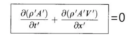
• MOmentum equation

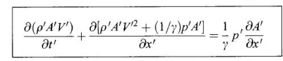
• Energy equation

STEP 2- FINITE DIFFRENTIAL EXPRESSIONS USING MacCORMACK'S EXPLICITE TECHNIQUE FOR THE NUMERICAL SOLUTION

To implement a finite-diffrence solution, we divide the x axis along the nozzle into a number of discrete frid poits,

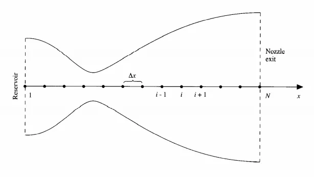
The frist grid point, labeled as point 1, is assumed to be in the resorvior. The points are evenly distributed along the x axis, with `Deltax` denoting the spacing between grid points the last point, namely, that at the nozzle exit, is denoted by N; we have a total number of Ngrid points distributed along the axis.Point i is simply an arbitary grid point, with points i-1 and i+1 as yhe adjecent points.

MacCormack's technique is preddictor -corrector method. in the time marchig approch, remember that we know the fluid field variable at time t, and we use the diffrence equation to solve explicitebfor gthe variable at time `t+Deltat`.

NON CONSERVATION FORM

Frist we consider the predictor step, we set up the spatial derivatives as forward diffrences

1.CONTINUITY EQUATION:-

2.MOMENTUM EQUATION:-

3.ENERGY EQUATION:-

Using the above values we will obtain the predicted values of `rho, V and T`

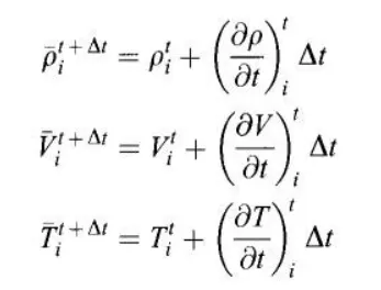
But these values are only frist order accurate. so we do tge corrector step to nake it second order accurate.

In the orrector step we frist obtain a predicted values of the time derivative at time `t+Deltat.((del rho)/(del t))_(i,j)^(t+Deltat)` , by substituting the predicted values of `rho ,u and v` into the right side of the continuity equation, replacing the spatial derivatives with rearward diffrences.

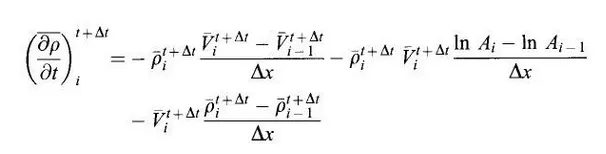
Likewise momentum and energy equations will be,

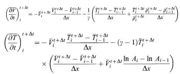
Using above eqations, the average time derivatives are

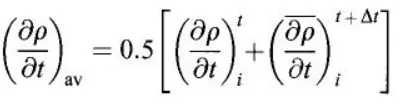
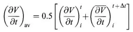
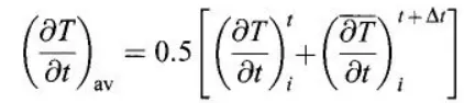
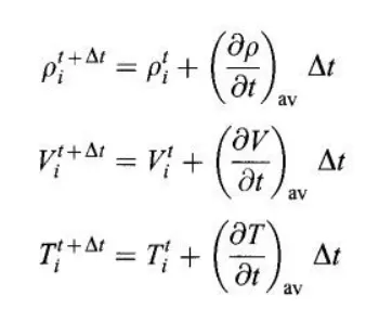
Then we can substitute the value into the below formula to find the corrected value of the flow -field variable at time `t+Deltat`

CONSERVATIONAL FORM

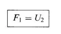
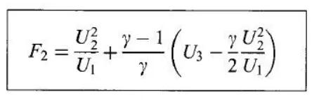
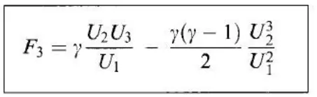
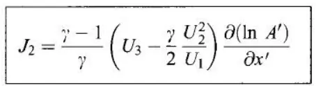
The eq. for quasi one diamension flow can be expressed in generic form. let us define the element of the solution vector U, the flux vector F, and the source term J as follows

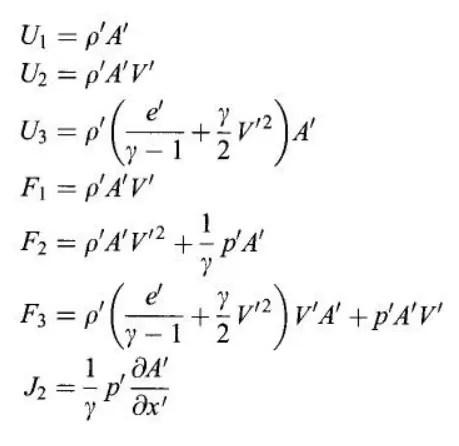
Frist finding the source vector with the above equations with iniial codition, then with them we can find the flux vectors.

PREDICTOR STEP:-

Then we set up the spatial derivatives as forward diffrences.

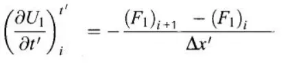
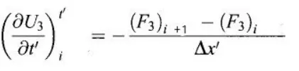
Then we find the predicted values of U1, U2 and U3

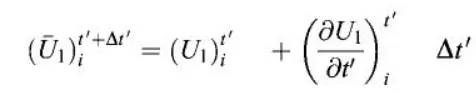
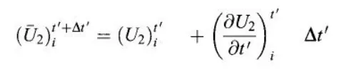
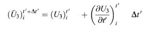
Using these values we will find the predicted values of the primitive variables.

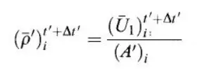
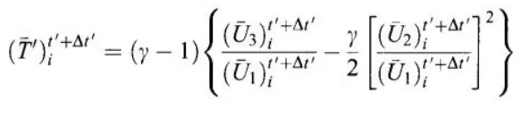
Now update the flux vector F1,F2,F3 with the new density, temperature and velocity

CORRECTOR STEP:-

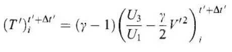
The predicted time derivatives of U1 U2 U3 are obtained above, and corrector time derivaties can be find using rearward diffrencing for the x derivatives.

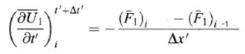
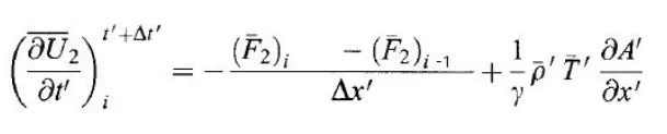
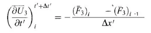
Then the avrage time derivatives are formed as follows:-

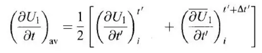
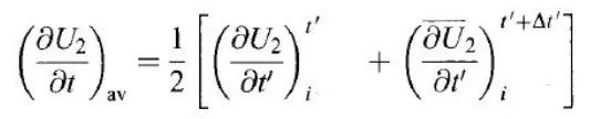
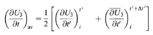
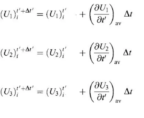
So, the final corrected values of U1 U2 U3 will become

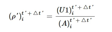
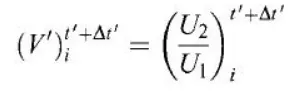
Finally the corrected values of the primitivr variable are obtained by decoding U1 U2 U3obtained above.

STEP 3 :- SETTING THE TIME STEP CALCULATION, INITIAL AND BOUNDARY CONDITIONS

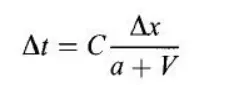
Time step can be calculated using the following formula:-

Where,

C= courant number

a= speed of sound

V- velocity

`Deltax` =Distance between 2 consective points.

NON CONSERVATIVE FORM

Nozzle shape:-

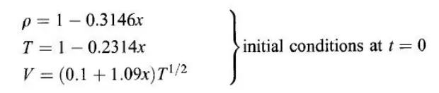
Initial conditions:-

initial conditions:-

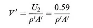
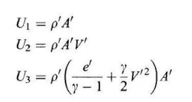
Boundary condition at inflow:-

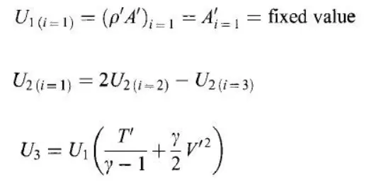
Boundary condition at outflow:-

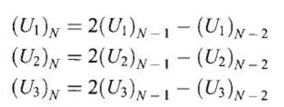
CODE:-

MAIN CODE

close all
clear all
clc

%inputs
L=3;
n=31;
dx=L/(n-1);
C=0.5;
nt=1400;
gamma=1.4;

%NON-CONSERVATIVE FORM
tic
[x,dt,rho,v,T,p,M,flow_rate_n,nt_grid,n_iter] = non_conservative_form(L,n,C,dx,nt);
toc
time_nc=toc;

fprintf('Time reqired for execution for non conservative form=%0.4gs',time_nc)


%CONSERVATIVE FORM
tic
[dt,rho,T,p,M,v,flow_rate_c,m_analytical,n_iter,tolerance]=conservative_form(L,n,C,dx,nt,gamma);
toc
time_con=toc;

fprintf('Time reqired for execution for conservative form=%0.4gs',time_con)

figure(7)
plot(x,flow_rate_n)
hold on
plot(x, flow_rate_c)
hold on
plot(x,m_analytical)
legend('non conservative form','conservative form','analytical solution')

FUNCTION CODE FOR NON-CONSERVATIVE:-

function [x,dt,rho,v,T,p,M,flow_rate_n,nt_grid,n_iter] = non_conservative_form(L,n,C,dx,nt);
L=3;
n=31;
dx=L/(n-1);
C=0.5;
nt=1400;
gamma=1.4;
x=linspace(0,L,n);
rho=1-0.3146*x;
T=1-(0.2314*x);
v=(0.1+1.09*x).*T.^0.5;
A=1+2.2*(x-1.5).^2;
gamma=1.4;
throat=(n+1)/2;
nt_grid=linspace(1,nt,nt);
initial_flow= rho.*v.*A;
flow_rate_old=0;
tolerance=1e-4;
error=999;
n_iter=1;
%analytical mass flow rate
m_analytical=0.579*ones(n);

  for m=1:n
    dt_x(m)=C*(dx/(T(m)^(1/2)+v(m)));
  endfor
  %time step
    dt=min(dt_x);
    
for k=1:nt
    
    rho_old=rho;
    T_old= T;
    v_old=v;
   
   % predictor method
   %predictor method using forward difference
   for i= 2:n-1
    dvdx=(v(i+1)-v(i))/dx;
    drhodx=(rho(i+1)-rho(i))/dx;
    dT_dx=(T(i+1)-T(i))/dx;
    dlogA_dx=(log(A(i+1))-log(A(i)))/dx;
    % continuity eq
    
    drhodt_p(i)= -rho(i)*dvdx-rho(i)*v(i)*dlogA_dx-v(i)*drhodx;
    
    % momentum eq
    
    dvdt_p(i)= -v(i)*dvdx-(1/gamma)*(dT_dx+(T(i)/rho(i))*drhodx);
    
    %energy eq    
    
    dTdt_p(i)= -v(i)*dT_dx-(gamma-1)*T(i)*(dvdx+(v(i)*dlogA_dx));

    
    %predictor solution step
    rho(i)= rho(i)+drhodt_p(i)*dt;
    v(i)= v(i)+dvdt_p(i)*dt;
    T(i)=T(i)+dTdt_p(i)*dt;
  endfor
     %correction step
  for i=2:n-1
    dvdx=(v(i)-v(i-1))/dx;
    drhodx=(rho(i)-rho(i-1))/dx;
    dT_dx=(T(i)-T(i-1))/dx;
    dlogA_dx=(log(A(i))-log(A(i-1)))/dx;
    % continuity eq
    
    drhodt_c(i)= -rho(i)*dvdx-rho(i)*v(i)*dlogA_dx-v(i)*drhodx;
    
    % momentum eq
    
    dvdt_c(i)=-v(i)*dvdx-(1/gamma)*(dT_dx+(T(i)/rho(i))*drhodx);
    
    %energy eq    
    
    dTdt_c(i)= -v(i)*dT_dx-(gamma-1)*T(i)*(dvdx+(v(i)*dlogA_dx));
 endfor   
     %avrage time derivation
    
    dvdt=0.5*(dvdt_p+dvdt_c);
    dTdt=0.5*(dTdt_p+dTdt_c);
    drhodt=0.5*(drhodt_p+drhodt_c);

    %final  step 
 for j=2:n-1
 
   rho(j)= rho_old(j)+drhodt(j)*dt;
   v(j)= v_old(j)+dvdt(j)*dt;
   T(j)=T_old(j)+dTdt(j)*dt;
 
 end
   %inlet boundary comditions
    
   v(1)=2*v(2)-v(3);
   
   %outlet boundary conditions
   v(n)=2*v(n-1)-v(n-2);
   rho(n)=2*rho(n-1)-rho(n-2);
   T(n)=2*T(n-1)-T(n-2);
   
   %calculating pressure (p), mach number (M) & mass flow rate 
   p=rho.*T;
   M=(v./((T).^0.5));
   
   flow_rate_n=rho.*v.*A;
   
   %capturing floe field st thorath for each time step
   rho_throat(k)=rho(throat);
   v_throat(k)=v(throat);
   T_throat(k)=T(throat);
   p_throat(k)=p(throat);
   M_throat(k)=M(throat);
      
      flow_rate_throat(k)= flow_rate_n(throat);
      
      error= max(abs(flow_rate_n-flow_rate_old));

      if error>tolerance
        n_iter=n_iter+1;
        flow_rate_old=flow_rate_n;   
    endif
      figure(1)
      % non diamensional mass flow distribution across the nozzle at diffetrnt time step
      % compared with analytical mass flowrate solution
      if k==50
        plot(x, flow_rate_n,'Linewidth',2);
        hold on 
        else if k==100
        plot(x, flow_rate_n,'Linewidth',2);
        hold on       
        
      else if k==150
        plot(x, flow_rate_n,'Linewidth',2);
        hold on 
      else if k==300
        plot(x, flow_rate_n,'Linewidth',2);
        hold on 
        
      else if k==700
        plot(x, flow_rate_n,'Linewidth',2);
       hold on
       
        plot(x,m_analytical,':');
        hold on
        plot(x,initial_flow,'--');
        
        legend('50Deltat','100Deltat','200Deltat','400Deltat','700Deltat','analytical solution','initial flow rate');
        title('non diamensional mass flow distribution across the nozzle at different time step before steady state non conservative form');
        xlabel('non diamensional x/L');
        ylabel('mass flow in non conservative form')
      
      end
    end
  end
end
end
    endfor
    %plotting steady state values 
figure(2)
title(sprintf('steady state values flow field variables in non conservation form , number of time step=%d',k))
subplot(5,1,1)
plot(x,M,'b','Linewidth',2);
xlabel('non diamensional length');
ylabel('M');
legend('mach number')

subplot(5,1,2)
plot(x,v,'r','Linewidth',2);
xlabel('non diamensional length');
ylabel('V/a_o');
legend('non diamensional velocity')

subplot(5,1,3)
plot(x,rho,'b','Linewidth',2);
xlabel('non diamensional length');
ylabel('rho/rho_o');  
legend('non diamensional density');

subplot(5,1,4)
plot(x,T,'y','Linewidth',2);
xlabel('non diamensional length');
ylabel('T/T_o');
legend('non diamensional temprature');

subplot(5,1,5)
plot(x,p,'b','Linewidth',2);
xlabel('non diamensional length');
ylabel('p/p_o'); i, 
legend('non diamensional pressure');


figure(3)
%time variation
plot(nt_grid,M_throat,'Linewidth',2)
hold on

plot(nt_grid,rho_throat,'Linewidth',2)
hold on

plot(nt_grid,v_throat,'Linewidth',2)
hold on

plot(nt_grid,T_throat,'Linewidth',2)
hold on

plot(nt_grid,p_throat,'Linewidth',2)
     
     legend('Mach Number','Non diamensional density','Non diamensional velocity','Non diamensional temprature','non diamensional pressure')
     xlabel('Number of time step')
     title('timewise variation of non diamensional flow field variables at throat in non conservation form')
end

FUNCTION CODE FOR CONSERVATIVE :-

function [dt,rho,T,p,M,v,flow_rate_c,m_analytical,n_iter,tolerance]=conservative_form(L,n,C,dx,nt,gamma);

L=3;
n=31;
dx=L/(n-1);
C=0.5;
nt=1400;
gamma=1.4;
x=linspace(0,L,n);
A=1+2.2*(x-1.5).^2;

gamma=1.4;
throat=(n+1)/2;
nt_grid=linspace(1,nt,nt);

m_analytical=0.579*ones(n);
n_iter=1;
%initial mass flow
U2_i=0.59;
flow_rate_old=0;
tolerance=1e-4;
error=999;

%analytical mass flow rate
for i=1:n
  if x(i)>=0 && x(i)<=0.5
  
  rho(i)=1.0;
  T(i)=1.0;
  
  else if x(i)>=0.5 && x(i)<=1.5
  
  rho(i)=1.0-(0.366*(x(i)-0.5));
  T(i)=1.0-(0.167*(x(i)-0.5));
  
  else if x(i)>=1.5 && x(i)<=3.5
  
  rho(i)=0.634-(0.3879*(x(i)-1.5));
  T(i)=0.833-(0.3507*(x(i)-1.5));
  endif
  endif
  endif
endfor
for j=1:n

    v(j)=U2_i/(rho(j)*A(j));
    U1(j)=(rho(j)*A(j));
    U2(j)=(rho(j)*A(j)*v(j));
    U3(j)=rho(j)*A(j)*((T(j)/(gamma-1))+(0.5*gamma*v(j)*v(j)^2));
end
  for m=1:n
    dt_x(m)=C*(dx/(T(m)^(1/2)+v(m)));
  endfor
  %time step
    dt=min(dt_x);
    U2_initial= U2;
    
for k=1:nt
    
    U1_old=U1;
    U2_old= U2;
    U3_old=U3;
   
%flux 
F1=U2;
F2=((U2.^2)./(U1))+(((gamma-1)/gamma).*(U3-((gamma/2).*(((U2.^2)./U1)))));
F3= ((gamma.*U2.*U3)./U1)-(gamma.*(gamma-1)/2)*((U2.^3)./U1.^2);

   % predictor method
   %predictor method using forward difference
   for i= 2:n-1
    dF1_dx=(F1(i+1)-F1(i))/dx;
    dF2_dx=(F2(i+1)-F2(i))/dx;
    dF3_dx=(F3(i+1)-F3(i))/dx;
    
    % continuity eq
    
    dU1_dt_p(i)= -dF1_dx;
    
    % momentum eq
    
    J2(i)=(1/gamma)*rho(i)*T(i)*((A(i+1)-A(i))/dx);
    dU2_dt_p(i)= -dF2_dx+J2(i);
    
    %energy eq    
    dU3_dt_p(i)= -dF3_dx;
    
    
    %predictor solution step
    U1(i)= U1(i)+dU1_dt_p(i)*dt;  
    U2(i)= U2(i)+dU2_dt_p(i)*dt;
    U3(i)= U3(i)+dU3_dt_p(i)*dt;
  endfor
     %update initial values
     
     rho= U1./A;
     v=U2./U1;
     T=(gamma-1).*((U3./U1)-(0.5*gamma.*v.^2));
     p=rho.*T;
     F1=U2;
     F2=((U2.^2)./(U1))+(((gamma-1)/gamma).*(U3-((gamma/2).*(((U2.^2)./U1)))));
     F3= ((gamma.*U2.*U3)./U1)-(gamma.*(gamma-1)/2)*((U2.^3)./U1.^2);
     
     %correction step
     
  for j=2:n-1
    dF1_dx=(F1(j)-F1(j-1))/dx;
    dF2_dx=(F2(j)-F2(j-1))/dx;
    dF3_dx=(F3(j)-F3(j-1))/dx;

    % continuity eq
    
    dU1_dt_c(j)=-dF1_dx;    
    % momentum eq
    
   J2(j)=(1/gamma)*rho(j)*T(j)*((A(j)-A(j-1))/dx);
    dU2_dt_c(j)= -dF2_dx+J2(j);
    
    %energy eq    
  dU3_dt_c(j)= -dF3_dx;
       
 endfor   
     %avrage time deriflow_rate_cation
    
    dU1_dt_avg=0.5*(dU1_dt_p+dU1_dt_c);
    dU2_dt_avg=0.5*(dU2_dt_p+dU2_dt_c);
    dU3_dt_avg=0.5*(dU3_dt_p+dU3_dt_c);
    %final  step 
   for m=2:n-1
   U1(m)= U1_old(m)+dU1_dt_avg(m)*dt;
   U2(m)= U2_old(m)+dU2_dt_avg(m)*dt;
   U3(m)= U3_old(m)+dU3_dt_avg(m)*dt;
   %inlet boundary comditions
    end
  U1(1)=rho(1)*A(1);
  U2(1)=2*U2(2)-U2(3);
  v(1)=U2(1)/(rho(1)*A(1));
  U3(1)= U1(1)*((T(1)/(gamma-1))+((gamma*0.5)*v(1)^2));  
   %outlet boundary conditions
   U1(n)=2*U1(n-1)-U1(n-2);
   U2(n)=2*U2(n-1)-U2(n-2);
   U3(n)=2*U3(n-1)-U3(n-2);
   
   %calculating pressure (p), mach number (M) & mass flow rate 
   p=rho.*T;
   M=(v./((T).^0.5));
   
   flow_rate_c=rho.*v.*A;
   
   %capturing floe field st thorath for each time step
   rho_throat(k)=rho(throat);
   v_throat(k)=v(throat);
   T_throat(k)=T(throat);
   p_throat(k)=p(throat);
   M_throat(k)=M(throat);
      
      flow_rate_throat(k)= flow_rate_c(throat);
      
      error= max(abs(flow_rate_c-flow_rate_old));
     
     if error>tolerance
        n_iter=n_iter+1;
        flow_rate_old=flow_rate_c; 
      endif
      figure(4)
      % non diamensional mass flow distribution across the nozzle at diffetrnt time step
      % compared with analytical mass flowrate solution
      if k==50
        plot(x, flow_rate_c);
       hold on
       else if k==100
        plot(x, flow_rate_c);
        hold on
      else if k==200
        plot(x, flow_rate_c);
       hold on
       else if k==500
        plot(x, flow_rate_c);
        hold on
      else if k==700
        plot(x, flow_rate_c);
        hold on
        
        plot(x,m_analytical,':');
        hold on
        plot(x,U2_initial,'--');
      
      legend('50Deltat','100Deltat','200Deltat','400Deltat','700Deltat','analytical solution','initial flow rate');
        title('non diamensional mass flow distribution across the nozzle at different time step before steady state conservative form');
        xlabel('non diamensional x/L');
        ylabel('mass flow in conservative form')
       end
     end
   end
 end
end
endfor
  %plotting steady state values 
figure(5)
title(sprintf('steady state values flow field variables in conservation form , number of time step=%d',k))
subplot(5,1,1)
plot(x,M,'b','Linewidth',2);
xlabel('non diamensional length');
ylabel('M');
legend('mach number')

subplot(5,1,2)
plot(x,v,'r','Linewidth',2);
xlabel('non diamensional length');
ylabel('V/a_o');
legend('non diamensional velocity')

subplot(5,1,3)
plot(x,rho,'b','Linewidth',2);
xlabel('non diamensional length');
ylabel('rho/rho_o');  
legend('non diamensional density');

subplot(5,1,4)
plot(x,T,'y','Linewidth',2);
xlabel('non diamensional length');
ylabel('T/T_o');
legend('non diamensional temprature');

subplot(5,1,5)
plot(x,p,'b','Linewidth',2);
xlabel('non diamensional length');
ylabel('p/p_o');  
legend('non diamensional pressure');

figure(6)
%time variation
plot(nt_grid,M_throat)
hold on
plot(nt_grid,rho_throat)
hold on
plot(nt_grid,v_throat)
hold on
plot(nt_grid,T_throat)
hold on
plot(nt_grid,p_throat)

     legend('Mach Number','Non diamensional density','Non diamensional velocity','Non diamensional temprature','non diamensional pressure')
     xlabel('Number of time step')
     title('timewise variation of non diamensional flow field variables at throat in conservation form')
end

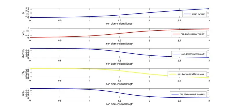
PLOTS

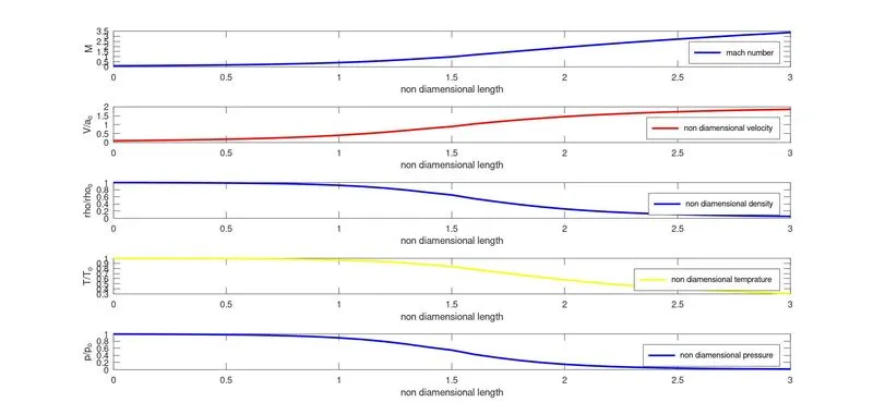
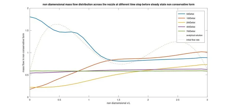
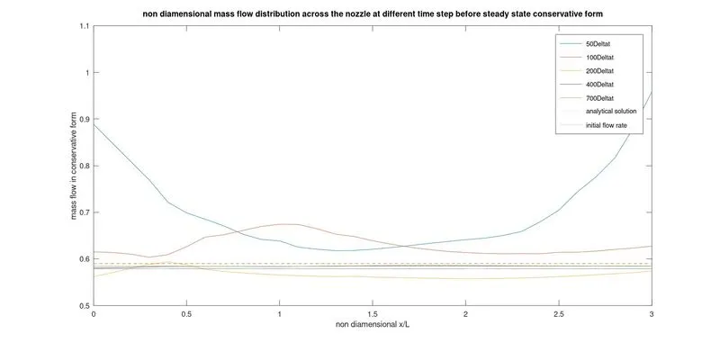
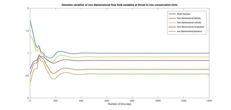
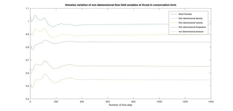
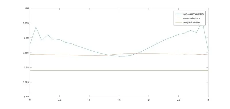
CONCLUSION :-

1. Better mass flow distribution is done in conservation form.
2. Non-conservation form is better for programming convenience because they are solved in term of primitive variables and their values are obtained directly.
3. But in conservation form equation are expressed in terms of flux variables and first solve solution vector then the primitive variables which makes things complex.
4. For accuracy also non-conservative is better due to the direct calculation of primitive variables.
5. While in conservation form primitive variables are calculated indirectly from flux variables. Increased number of calculations will lead to more errors.
6. This is the case when we take primitive valrables. But if we are taking Flux variables conservation form is better.
7. In non conservation form behavior of the residuals are good as compare to conservation form. The residuals decays faster in non conservation form when compared to conservation form.
8. The amount by which the residual decay is often used as an index 'quality' of the numerical algoritm. so the non conservation form is better.