Week 5: Project : Centrifugal pump simulation

Aim - Centrifugal Pump simulation in Converge 3.0

Introduction - Observing Performance plots for the pump at varying mass flow rates.

Centrifugal pump -

A centrifugal pump is a mechanical device designed to move fluid by means of the transfer of rotational energy from one or more driven rotors, called impellers. Fluid enters the rapidly rotating impeller along its axis and is cast out by centrifugal force along its circumference through the impeller's vane tips. The action of the impeller increases the fluid's velocity and pressure and also directs it towards the pump outlet. The pump casing is specially designed to constrict the fluid from the pump inlet, direct it into the impeller and then slow and control the fluid before discharge.

The impeller is the key component of a centrifugal pump. It consists of a series of curved vanes. These are normally sandwiched between two discs (an enclosed impeller). For fluids with entrained solids, an open or semi-open impeller (backed by a single disc) is preferred. Fluid enters the impeller at its axis (the 'eye) and exits along the circumference between the vanes. The impeller is on the opposite side to the eye. is connected through a drive shaft to a motor and rotated at high speed (typically 500-5000rpm). The rotational motion of the impeller accelerates the fluid out through the impeller vanes into the pump casing.

The pump casing consists of a volute and diffuser. The purpose in both designs is to translate the fluid flow into a controlled discharge at a pressure in a volute casing, the impeller is offset, effectively creating a curved funnel with an increasing cross-sectional area towards the pump outlet. This design causes the fluid pressure to increase towards the outlet.

Geometry -

• Geometry creation-
  • Geometry was Imported. Drag-Drop
  • 
  • 
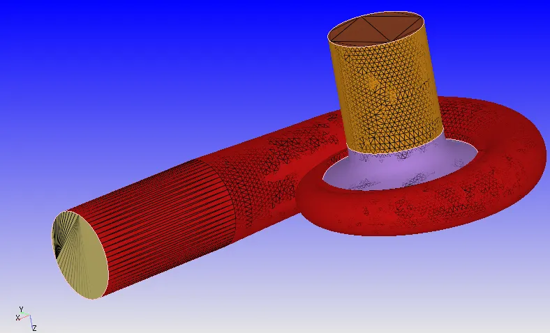
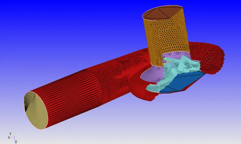
• Boundary Flagging
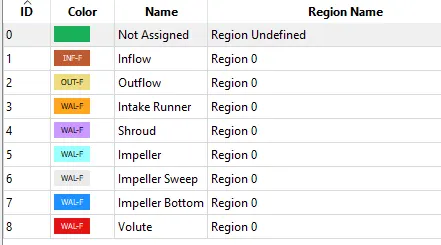
  • Boundaries were defined using the Boundary function
  • 8 different boundaries were defined as follows -
  • 

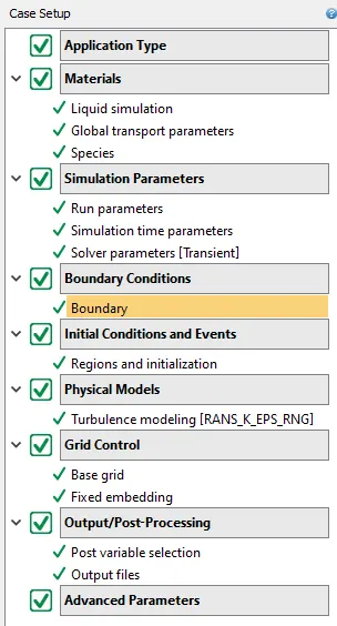
Case Setup

• Application type > Time-based
• Materials> Select "Liquid simulation"
  • Select H2O from predefined Liquid
  • Select H2O Species
• Simulation parameters
  • Run Parameters - Transient
  • Simulation time parameters - End time 0.2s
  • Solver parameters - Density-based NS solver
• Boundary conditions-parameters assigned as follows
  • Inlet - Inflow Type-101325.0Pa. 300K, H2O Species
  • Outlet - Outflow Type - Mass Flow rate
    • Case 1 - 130 kg/s . 300K. H2O Species
    • Case 2 - 156 kg/s . 300K. H2O Species
    • Case 3 - 180 kg/s . 300K. H2O Species
  • Intake runner and Shroud - Wall - Law of wall - Stationary Wall
  • Impeller, Impeller Sweep and Bottom - Wall - Law of wall - Rotating motion / Moving movement > Rotation rate - 12000 Degrees/s
  • Volute - Wall - Law of wall - Fixed movement
• Initial Conditions and Events
  • Region and initialization - Add Volumetric Region with H2Ospecies. Initial pressure-Inlet pressure - 101325.0Pa. 300K.
• Physical Models - Turbulence Model - RNG-k-e
• Grid Control
  • Base Grid - 0.012x0.012x0.012 m
  • Fixed Embedding
    • Boundary-Impeller- Permanent-Scale-2. Embed Layers 1
• Output/Post-processing
  • Time interval 3D O/p files - 0.002s
• Advanced Parameters
• 

Observations - After running the calculation on Cygwin following are the results observed in Paraview and Converge Line plotting tool. Kindly note the plots for all the 3 Cases.

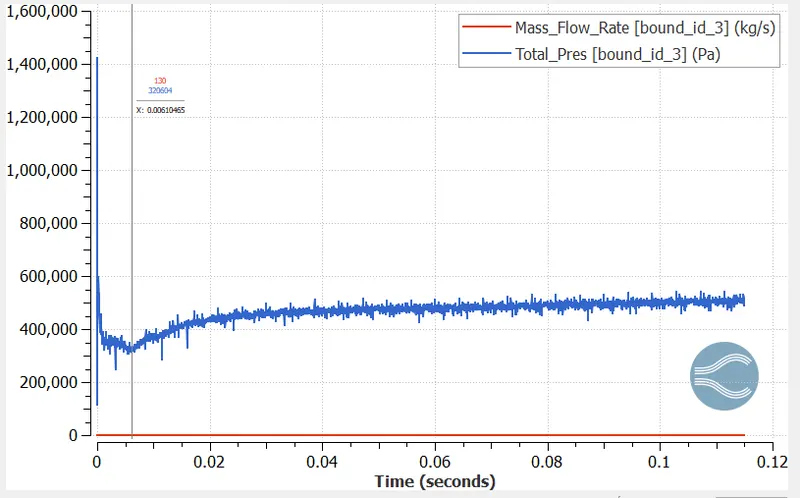
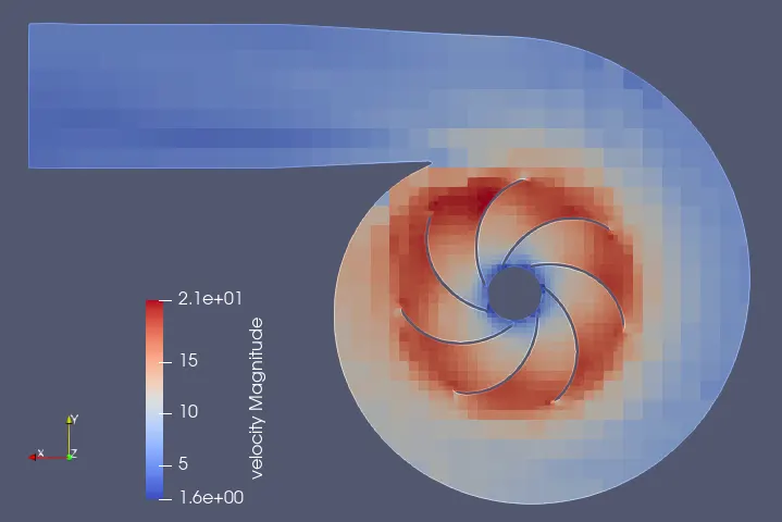
• Case 1 - 130Kg/s Mass flow rate -
  • Performance plot - Total Pressure vs Mass flow rate at the outlet
  • 
  • Velocity Contour
  • 
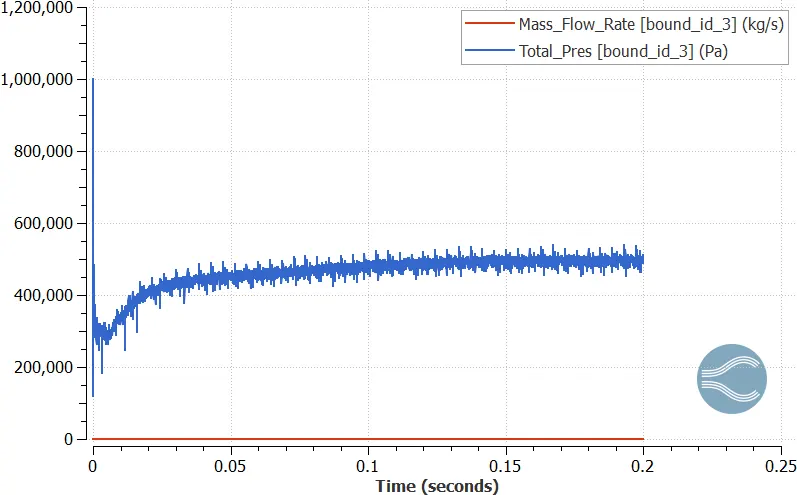
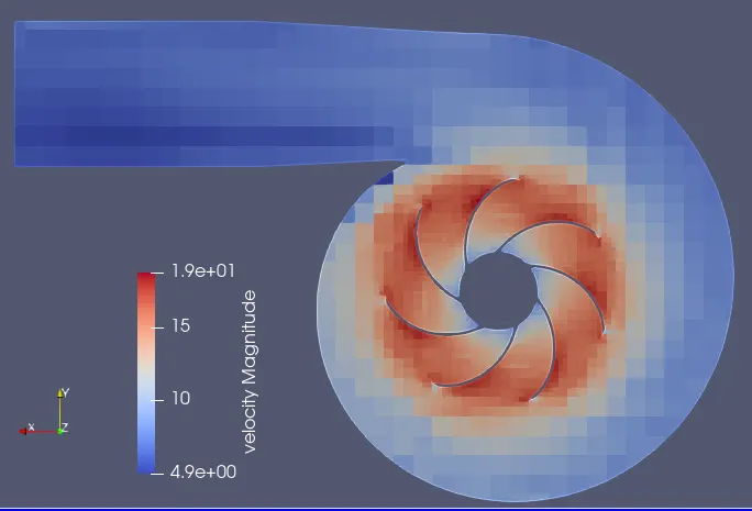
• Case 2 - 156Kg/s Mass flow rate -
  • Performance plot - Total Pressure vs Mass flow rate at the outlet
  • 
  • Velocity Contour
  • 
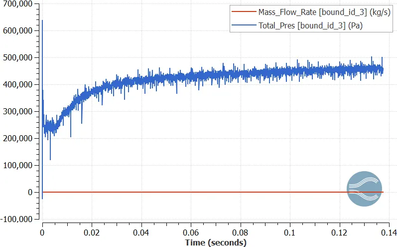
• Case 3 - 180Kg/s Mass flow rate -
  • Performance plot - Total Pressure vs Mass flow rate at the outlet
  • 
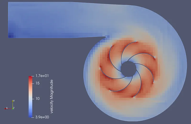
  • Velocity Contour -
  • 
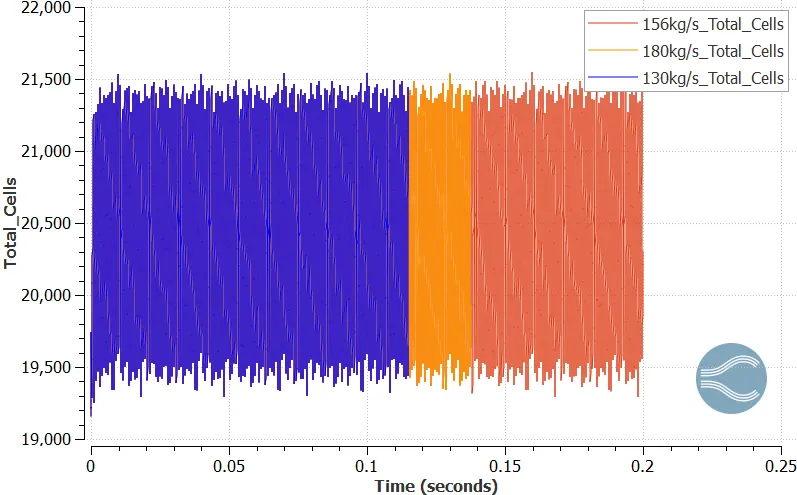
• Mesh -
  • Mesh Cell count -
  • 
• From the above plots, we observe that the mass flow rate throughout the pump is constant, the max pressure at the outlet can also be observed in the plots. The pressures, mass flow rate, and other quantities are noted from Converge line plotting tool and mentioned below for all the cases.

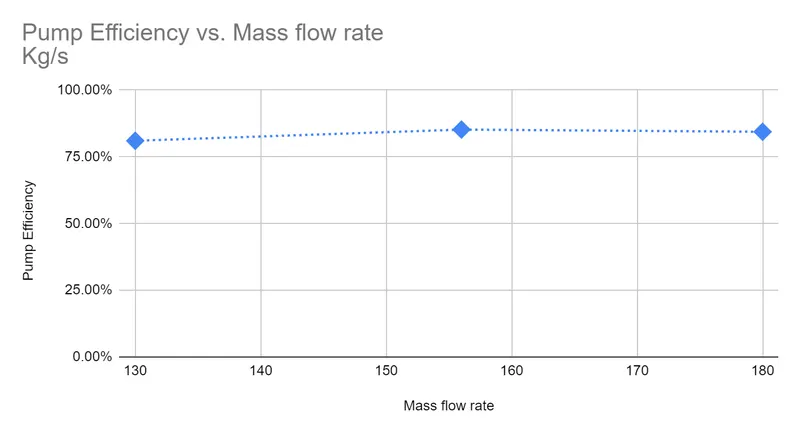
  • Mass flow rate	Outlet press	Inlet Press	Pressure Ratio	Head	Hydraulic power	Torque	Impeller speed	Angular velocity	Shaft power	Pump Efficiency
    Kg/s	Pa	Pa		m	Kw	Nm	deg/s	rad/s	Kw
    130	519000	101325	5.12	42.59	54.31	320	12000	209.44	67.02	81.04%
    156	496000	101325	4.90	40.25	61.58	345	12000	209.44	72.26	85.23%
    180	445000	101325	4.39	35.04	61.88	350	12000	209.44	73.30386	84.41%
• Calculations / Formulas
  • Pump Efficiency formula
  • Efficiency = ( Hydraulic power / shaft power ) * 100
  • Hydraulic power Kw = ( Mass flow rate m3/hr * Head in m ) / 367 ---- at outlet
  • Head = outlet pressure / (SG of water(1) * 0.0098)
  • Shaft power Kw = Torque * Angular velocity in rad/s ---- at the impeller

• Pump Efficiency plot / Performance curve

• Animation links-
  • AMR - https://youtu.be/Up_rY7ZlRXQ
  • Case 1 - https://youtu.be/PGJ-ptcL0Bo
  • Case 2 - https://youtu.be/useFJ4IWM7I
  • Case 3 - https://youtu.be/oRNXPQd_tDk

• Conclusion -

  In all the cases low-pressure zones can be observed at the eye of the impeller, velocity at the tip is maximum due to which low pressure reagion is created behind the tip which leads to cavitation on the impeller tip. The best efficiency 85% is observed in the 2nd case where the mass flow rate is 156kg/s. We also observe that as the mass flow rate increases the head obtained at the outlet decreases.