Week 1: Channel flow simulation using CONVERGE CFD

Aim - Flow-through Channel in Converge 3.0

Introduction - Observing the flow-through channel of dimnesion 0.1m x 0.01m x 0.01m(LxHxD) with 3 different mesh size.

Theory -

Geometry -

• Geometry creation -
  • Geometry was created using the Create function from the Geometry Dock
  • Create > Shape > Box > dx-0.1m, dy-0.01m, dz-0.01m
  • 
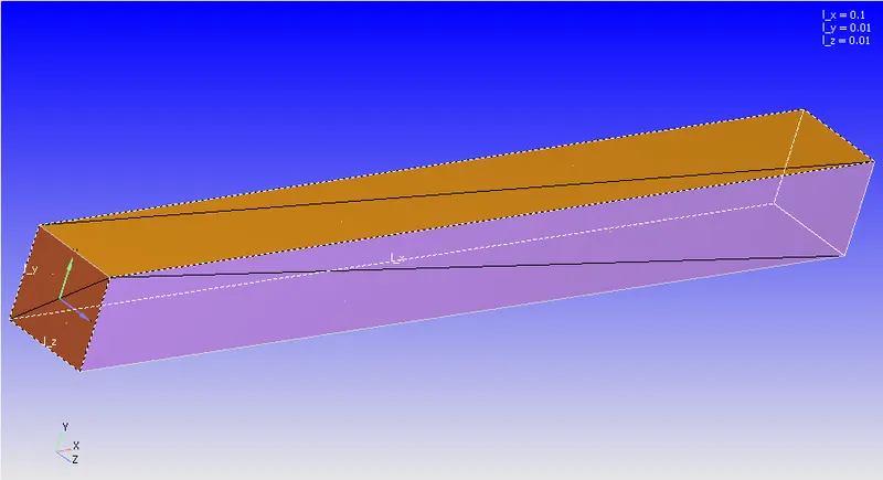
• Boundary Flagging
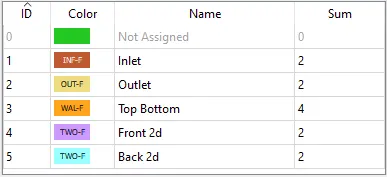
  • Boundaries were defined using the Boundary function
  • 5 different boundaries were defined as follows -
  • 

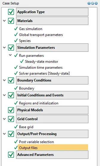
Case Setup -

• Application type > Time-based (For 2D Channel flow)
• Materials > Select Predefined mixture "Air"
  • O2 and N2 Gas species added
• Simulation parameters
  • Run Parameters - Select steady-state monitor > Add variables that are needed to be monitored(Velocity, Pressure, etc)
  • Simulation time parameters - End time > 15000 cycles
  • Solver parameters(SS) - Density-based NS solver
• Boundary conditions - parameters assigned as follows
  • Inlet - Inflow Type - 100001.0Pa, 300K, Air Species
  • Outlet - Outflow Type - 100000.0Pa, 300K, Air Species
  • Top Bottom - Wall - No-Slip Fixed wall
  • Front & Back - 2D
• Initial Conditions and Events
  • Region and initialization - Add Volumetric Region with Air species, Initial pressure = Inlet pressure = 100001.0Pa, 300K
• Physical Models - Default
• Grid Control -
  • Case I - Base Grid - dx = 2e-4m, dy = 2e-4m, dz = 2e-4m
  • Case II - Base Grid - dx = 1.5e-4m, dy = 1.5e-4m, dz = 1.5e-4m
  • Case III - Base Grid - dx = 1.2e-4m, dy = 1.2e-4m, dz = 1.2e-4m
• Output/Post prossessing
  • Time Interval 3D O/p files - 150cycs
• Advance Parameters

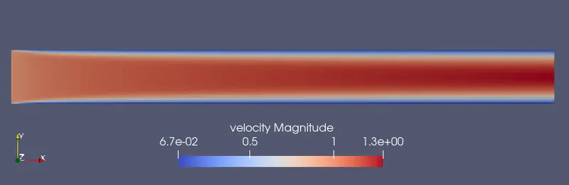
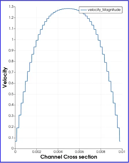
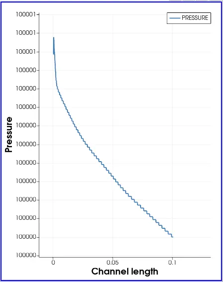
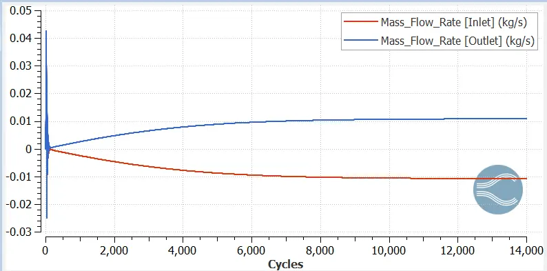
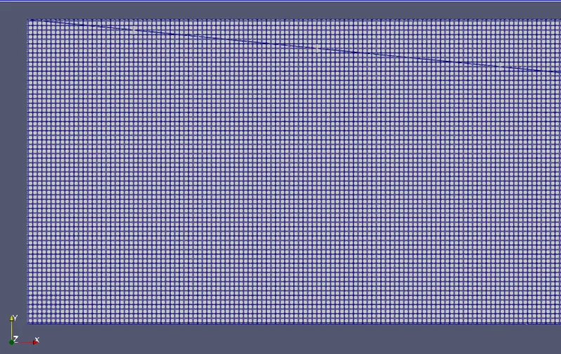
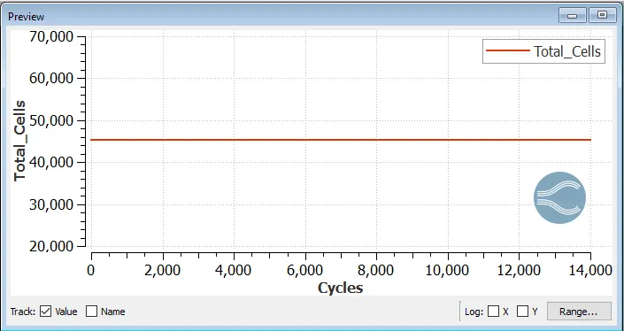
Observations - After running the calculation on Cygwin following are the results observed in Paraview and Converge Line plotting tool. The calculations were done with 3 different mesh sizes as mentioned below. At the start, a spike in the readings of velocity, pressure, etc is observed due to the pressure difference between Inlet and Outlet leading to a unidirectional flow through the channel. As the size of the base grind reduces the no cells increase and the results/No-Slip wall effect can be seen more clearly in the output.

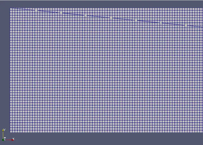
• Case I - Base Grid - dx = 2e-4m, dy = 2e-4m, dz = 2e-4m
  
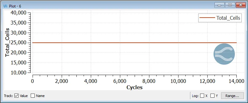
  • Mesh & Total cell count
  • 
  • 
  • Velocity at Inlet and Outlet
  • 
  • 
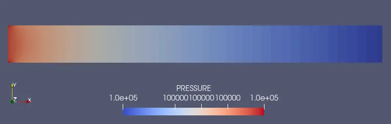
  • Pressure at Inlet and Outlet
  • 
  • 
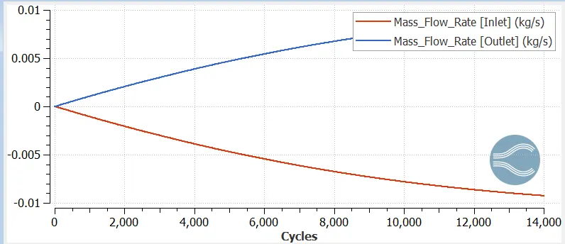
  • Mass flow rate at Inlet and Outlet
  • 
• Case II - Base Grid - dx = 1.5e-4m, dy = 1.5e-4m, dz = 1.5e-4m
  
  • Mesh & Total cell count
  • 
  • 
  • Velocity at Inlet and Outlet
  • 
  • 
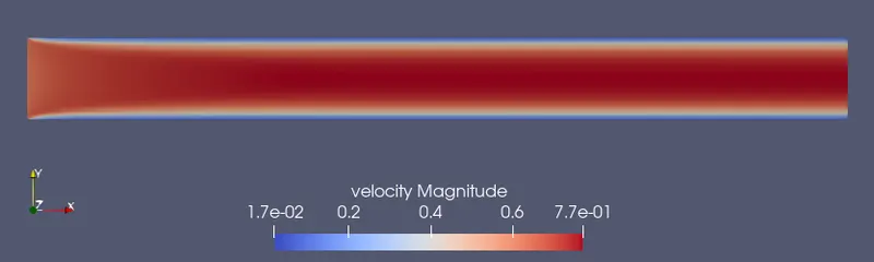
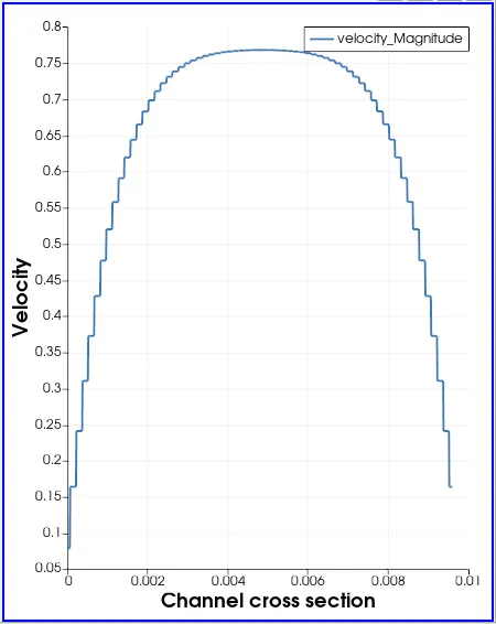
  • Pressure at Inlet and Outlet
  • 
  • 
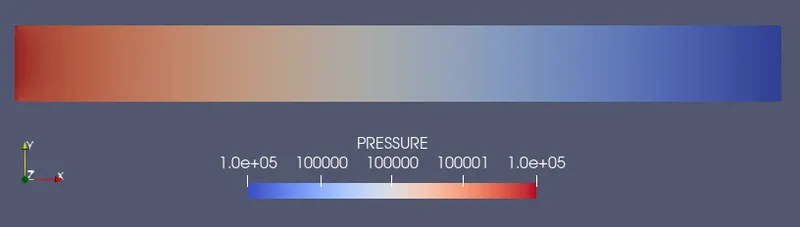
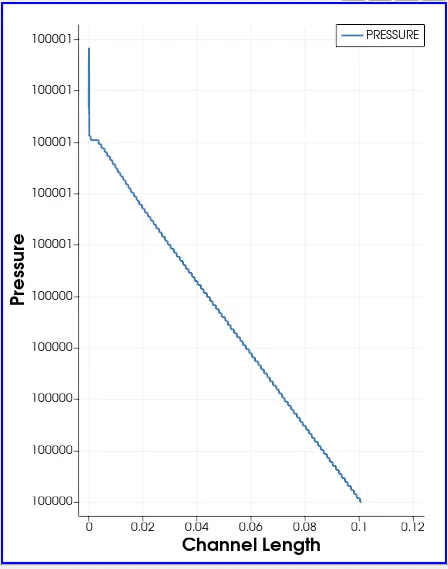
  • Mass flow rate at Inlet and Outlet
  • 
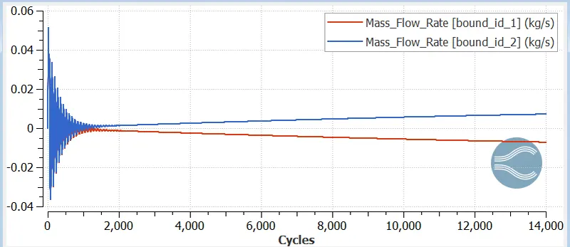
• Case III - Base Grid - dx = 1.2e-4m, dy = 1.2e-4m, dz = 1.2e-4m
  
  • Mesh & Total cell count
  • 
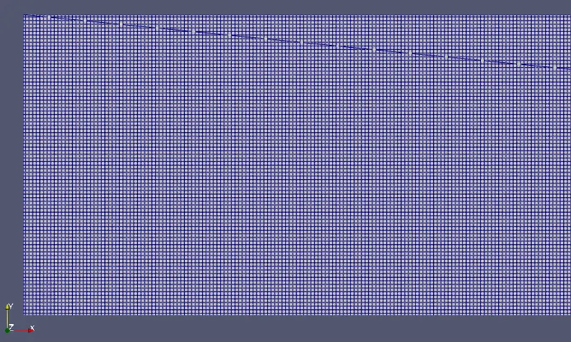
  • Velocity at Inlet and Outlet
  • 
  • 
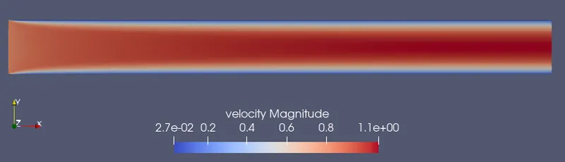
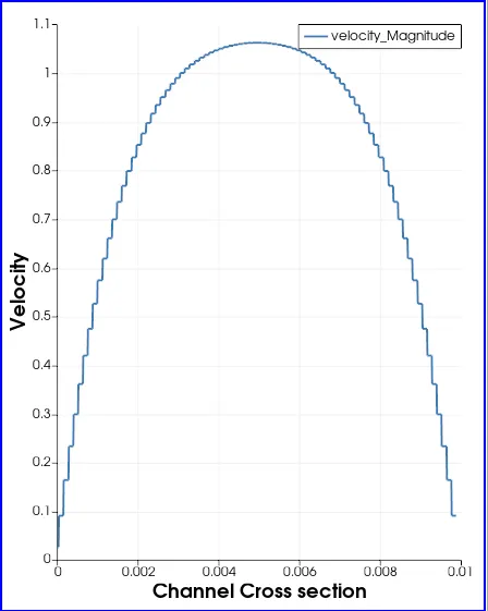
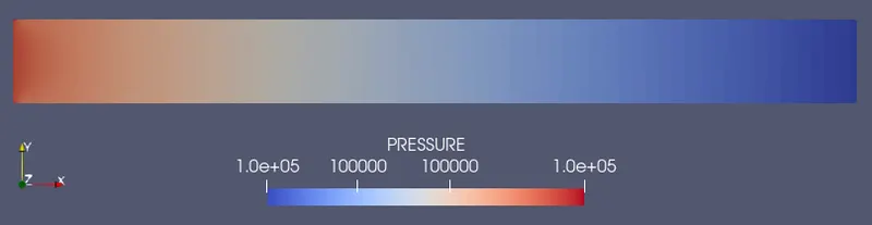
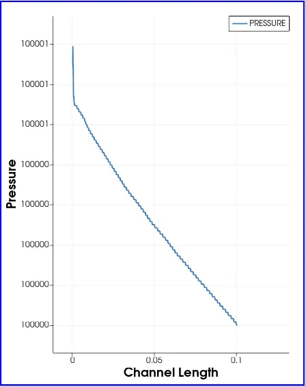
  • Pressure at Inlet and Outlet
  • 
  • 
  • Mass flow rate at Inlet and Outlet
  • 

Animation Link - https://youtu.be/l1i5sQ3Vp8E

Conclusion -

Velocity profile due to no-slip wall is clearly visible in all the cases. Max velocity can be seen along the center of the channel and at the top and bottom walls, the velocity is zero.

Flow can be observed from the High-pressure inlet to the Low-pressure outlet.

The mass flow rate plot indicates that mass flow through the inlet equals mass flow through the outlet. No accumulation mass inside the channel.