Week 5: Prandtl Meyer Shock problem

Aim: - To simulate steady-state subsonic and supersonic flow around convex corner and show Prandtl-Meyer expansion.

Objective: -

4. Discuss shock wave and different boundary condition used for shock flows.
5. Discuss the Prandtl-Meyer expansion Fan and it working.
6. To simulate flow with following conditions in the given model with convex corner at bottom.
   
   • Inlet Velocity = 680 m/s (Supersonic flow) and SGS parameter = 0.05
   • Inlet Velocity = 680 m/s (Supersonic flow) and SGS parameter = 0.01
   • Inlet Velocity = 680 m/s (Supersonic flow) and SGS parameter = 0.005
   • Inlet Velocity = 100 m/s (Subsonic flow) and SGS parameter = 0.05
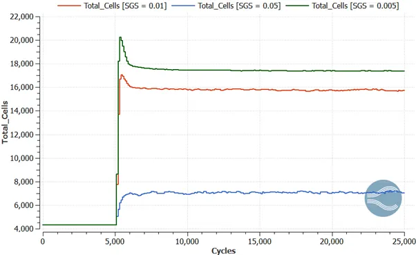
7. To plot and compare the result. Discuss the effect of SGS (Sub-Grid Scale) parameter on total number of Cell Count.

Theory: -

Shock Wave –

It is a type of propagating disturbance that moves faster than the local speed of sound in the medium. It carries energy and can propagate through a medium but is characterized by an abrupt, nearly discontinuous, change in pressure, temperature, and density of the medium.

In supersonic flows, additional increased expansion may be achieved through an expansion fan, known as a Prandtl–Meyer expansion fan.

There are 5 types of boundary condition, which are as follows: -

1. Dirichlet BC: This condition specifies the value that the unknown function needs to take on along the boundary of the domain.
2. Neumann BC: This condition when imposed on ODE or PDE, it specifies the values that the derivative of a solution is going to take on the boundary of the domain.
3. Robin BC: This condition consists of a linear combination of the values of the field and its derivative of the boundary. this condition is also known as impedance condition.
4. Mixed BC: It consists of applying different types of BC in different parts of the domain. It is important that BC must be applied on the whole boundary. The mixed boundary condition differs from the Robin condition because the latter consists of different types of boundary conditions applied to the same region of the boundary, while the mixed condition implies different types of boundary conditions applied to different parts of the boundary.
5. Cauchy BC: It is the condition on both the unknown field and its derivative. it differs from Robin condition because it implies the imposition of two constraints while robin condition implies only one constraint on the linear combination of unknown function and its derivative.

Boundary Condition used in Shock Flow –

Neumann Boundary condition are preferred over other in shock flow as thermodynamic properties can oscillates and values had to be extrapolated from the interior regions at each states rather than providing specifics values which could deaccelerate the convergence of solution.

Prandtl-Meyers Expansion fan –

It works on a centered expansion process that occurs when a supersonic flow turns around a convex corner. The fan consists of an infinite number of Mach waves, diverging from a sharp corner. these waves can be extended backwards to meet at a point. Each wave in the expansion fan turns the flow gradually.

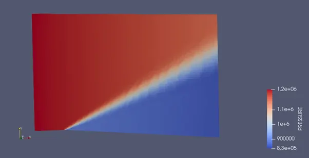
Across the expansion fan, the flow accelerates (velocity increases) and the Mach number increases, while the static pressure, temperature and density decrease. Since the process is isentropic, the stagnation properties (total pressure and total temperature) remain constant across the fan.

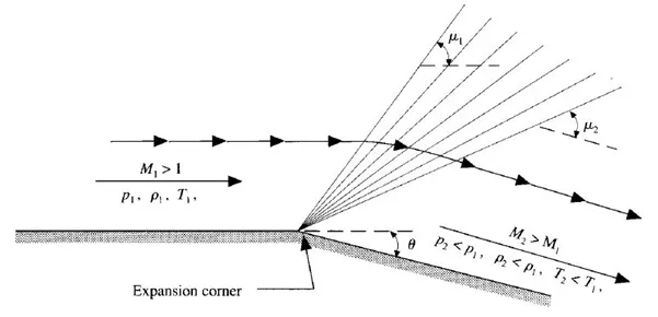
The Mach Line Number

`μ_1=sin^(-1) (1/M_1 ) and μ_2=sin^(-1) (1/M_2 )`

Prandtl–Meyer function

`ν(M) = √((γ+1)/(γ-1)) *tan^(-1) (√((γ-1)/(γ+1)*(M^2-1) ) - tan^(-1) (√(M^2-1))`

`θ= ν(M_2 ) - ν(M_1 )`

by using above two equations on can guess the Mach number associated with outlet if inlet Mach number and angle is Known.

Geometric Model: -

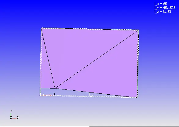
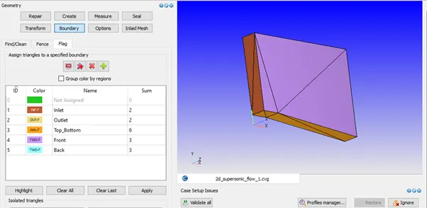
Case Setup: -

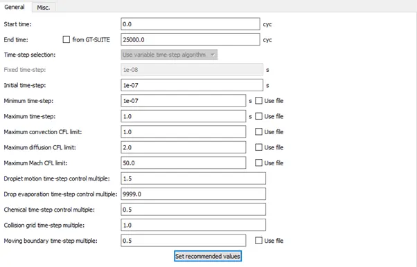
1. Time Based application type.
2. Gas simulation with Air as predefined mixture

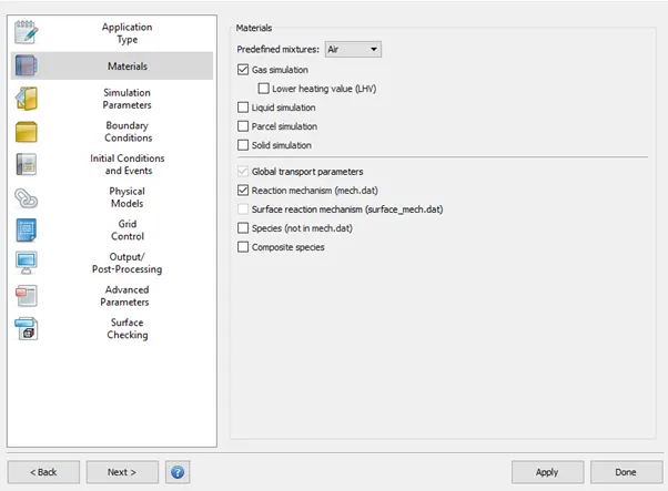
3. Pressure Based Steady State Solver is used with Compressible Gas Flow solver and PISO Navier-Stokes’s solver scheme.
4. The solution run for 25000 cycles with minimum time step of 1e-7 s and maximum up to 1 sec.

5. Boundary Condition:
   286. Inlet - Type = Inflow, Pressure = Zero normal gradient, Velocity = 680 m/sec (for Supersonic) and 100 m/sec (for Subsonic), Temperature = 286.1 K, Species = O2:0.23, N2: 0.77
   287. Outlet - Type = outflow, Pressure and Velocity = Zero normal gradient, Temperature = 300 K Species = O2:0.23, N2: 0.77
   288. Top-Bottom – Type = wall, slip Condition
   289. Front and Back- Type = 2D

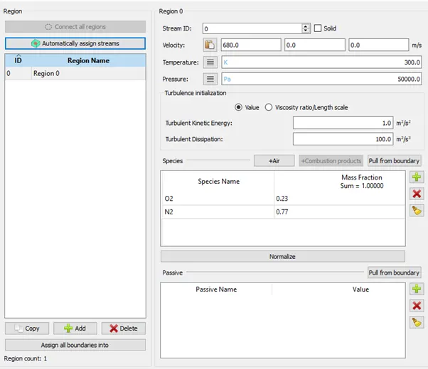
6. Volumetric Region are initialized with Temperature 300, Pressure 50,000 Pa, Velocity equal to inlet Velocity and mass fraction of O2: 0.23 and N2: 0.77. The boundaries are assigned their region type.

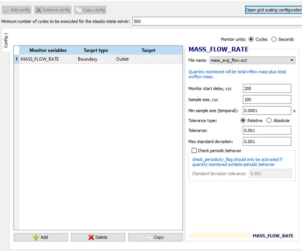
7. A Mass-flow-rate monitor is set to monitor mass flow rate during simulation.

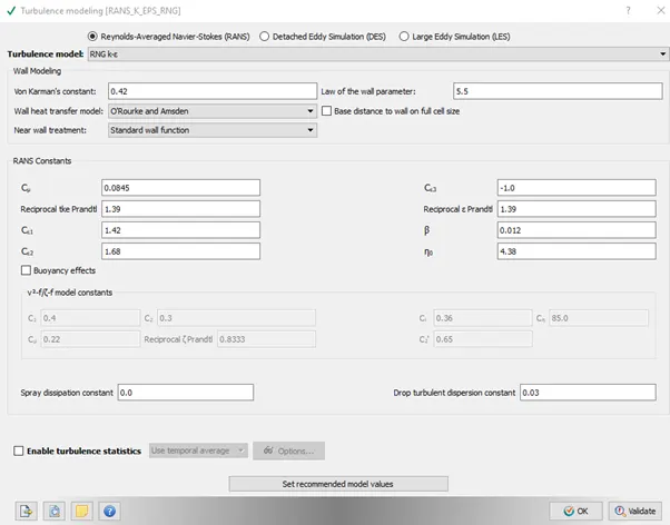
8. RNG K-epsilon is used for turbulence modelling with recommended values.

9. Base grids of 0.8 m are generated for all axis. Adaptive Mesh Refinement is also added on the basis of temperature.

Here sub-Grid criterion is changed according the requirement.

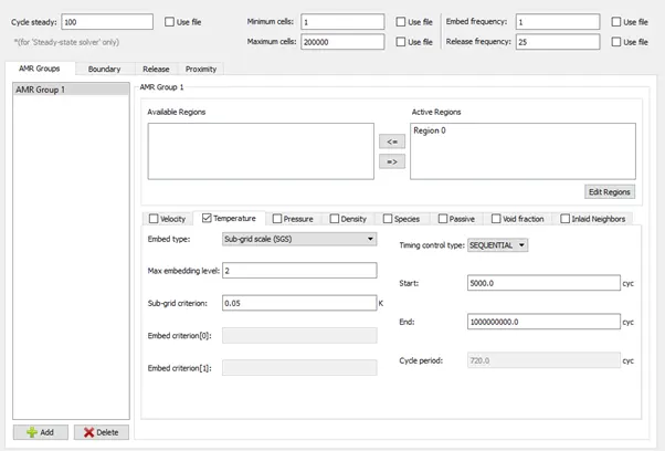
10. 3D output data is written after every 125 cycles.

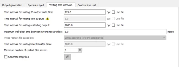
11. The input files are exported to a folder to further solving.

Solving using Cygwin:

An executable “mpiexec.exe” is placed with the exported folder. The Cygwin directory is navigated to the above saved folder and following code is entered to solve the problem.

mpiexec.exe -n 2 "C:\Program Files\Convergent_Science\CONVERGE\3.0.16\bin\intelmpi\converge.exe" restricted </dev/null> logfile &

where address in quotes gives the path of folder containing input file exported earlier.

Post-Processing:

Post-Processing is done with the help of Converge CFD post processing tab –

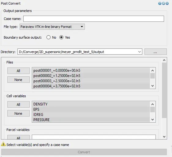
with these the output 3D data is converted in ‘.vtm’ file and contours and animations are prepared though ParaView.

Results: -

Initial Mesh

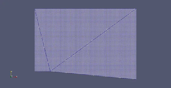
Case 1: Inlet Velocity = 680 m/s (Supersonic flow) and SGS parameter = 0.05

final Mesh

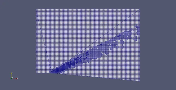
Mesh with AMR animation

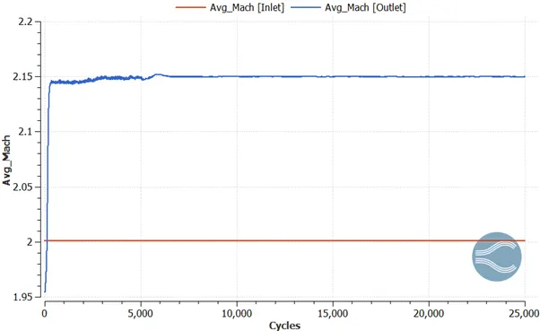
Mach Number

Pressure Contour

Velocity Animation

Case 2: Inlet Velocity = 680 m/s (Supersonic flow) and SGS parameter = 0.01

final Mesh

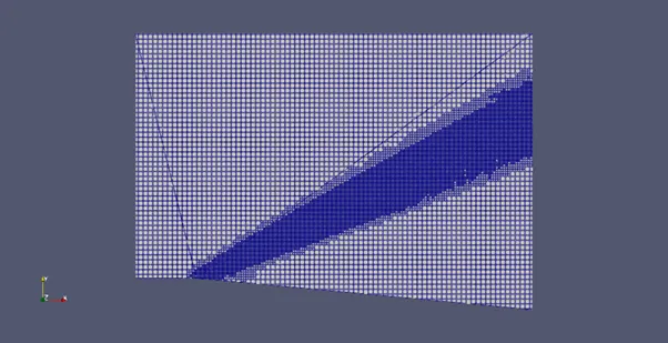
Mesh with AMR animation

Mach Number

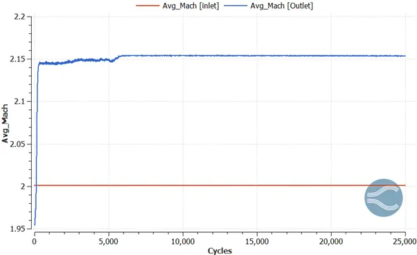
Pressure Contour

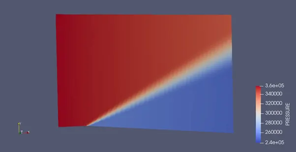
Velocity Animation

Case 3: Inlet Velocity = 680 m/s (Supersonic flow) and SGS parameter = 0.005

final Mesh

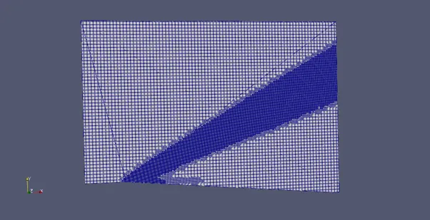
Mesh with AMR animation

Mach Number

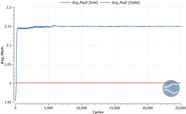
Pressure Contour

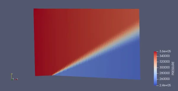
Velocity Animation

Case 4: Inlet Velocity = 100 m/s (Subsonic flow) and SGS parameter = 0.05

final Mesh

Mesh with AMR animation - No change through out the simulation as expansion does not happens, hence requirements for refinement not fulfilled .

Mach Number

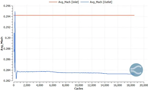
Pressure Contour

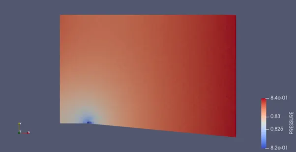
Velocity Contour

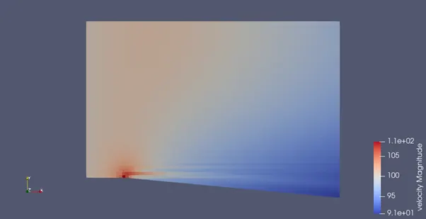
Cell Count Comparison –

Conclusion: -

• As SGS decreases the accuracy of the solution increases and calculation time also increases.
• SGS 0.05 gives the best result of 2.153 Mach Number at outlet boundary.
• Prandtl-Meyer Expansion Fan only works with supersonic streams not sub sonic as velocity of 2 Mach shows the phenomena but not with 100 m/sec.
• Number of cells increase with decrease in SGS parameter as refinement becomes more sensitive with lower SGS.