Week 5: Prandtl Meyer Shock problem
Aim-.To Simulate the Prandlt Meyer shock problem for both supersonic abd subsonic for different SGS scale.
objectives-
To determine the effect of SGS temperature value(0.01,0.05,0.1) on the shock location and on the cell count.
Theroy-
Shock wave is the propagating the distrubance in the medium . When the velocity of the propagating wave is more than the velocity of the sound in the medium the shock waves are generated. It consists of infinte number of weak mach waves. and its charactersised by abrut change in the trmperature,pressure ,velocity and density.
Meyer Prandlt Expansion
When the supersonic waves flows around the sharp the corner of the wedge shape or around the convex shape there is sudden expansion of waves take place .This expansion is called Prandlt Meyer expansion. When the flow turns the forward the waves are extended back meet at the point.since there is increase in the velocity the static preesure, density, temperature decreases. and as the process is isoentropic the total pressure and the total temperature remains constant.
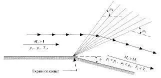
Different types of Boundary condtion for the shock waves
1.Dirchlet Boundary condtion- In this the value of the function is directly imposed on the boundary surface.
Y=f in this case the inlet velocity 680m/sec is the value applied at the inlet.
2.Neuman boundary condtion-this condtion involves application of the devative normal of the function to the boundary surface.in this cases all the output values are taken as the neuman and as zero gradient(i.e dp/dx=0,dv/dx=0) becuse at the outlet all the values are extraplotted from the interior condtion .
3.Robin Boundary condtion-Its combination of Dirchlet boundary and the neuman boundary condtion.
case set up-
1.first we import geometry stl file in to the converge studio.
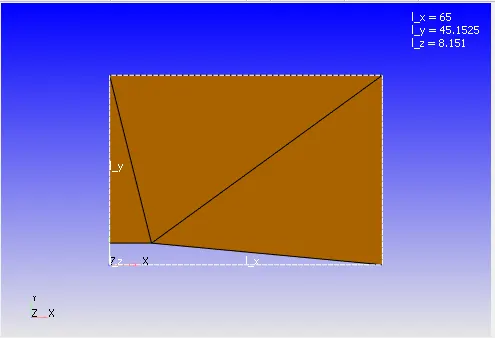
2.Material
after the formation of the geometry we take air as the flowing materia.
3.Boundary condtion
after setting materila now we assign the boundary condtion the left of the step is given as the inlet and the right face of the step is given as the outlet .and we apply the inlet velocity of 680 m/sec and the temparature of 286k and the spieces of air .and the outlet the pressure and the velocity are given as zero gradient as they are extraplotted fronm the inlet condtion. and top face and bottom face we give as the wall .at the walls the the grid size length is going to be greater than the acutual leength hence we give slip condtion.
3.Intial condtion
Spieces of air with masss fraction of O2 as 0.77 and the mass fraction of the N2 as 0.23 at 300k and at 101325pa.
4.Grid size and Adpative mesh refinement- we are using the grid size of 0.8 for all cases . since around the shock wave the flow parameters are going to change aburtly hence in order to capture them we use AMR mesh technique which consists of subgrid scale(SGS) when the seconder order of flow paramters exceeds the subgrid scale value the AMR is going the mesh the area arond the shock waves for example when our given SGS scale is 0.005 but the one of the second order of flow quanties example temperature is .1k then AMR is going to refine the area around the shock waves .and the size of the refinement cell is determined using the formula =base grid size/(2^n) where n is the number of embeded layers. in this case n=2
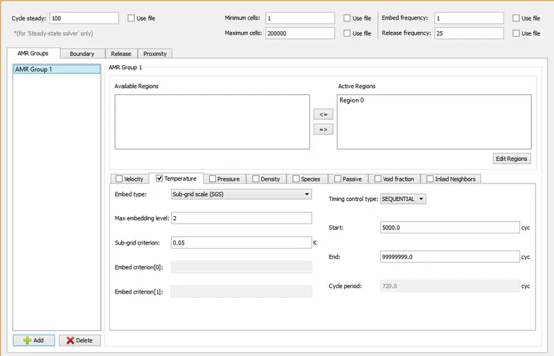
5.Simulation and Time parameters
we use steady state solver with full hydrodynamic as there are no moving parts if moving parts involves the we have to select the transient solver.
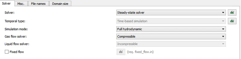
we have the simulation time parameters as
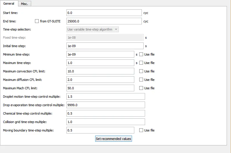
the simulation time starts from 0 cycles (here cycles for steady state and sec for transient solver)the end of the simulation depends on the solution attaing the convergence i.e the steady state starts monntoring for every cycles ande for every 1000 cycles it will check the tolerance of the average parameters for an example for 1000 cycles the average velocity is 2.25m/sec and for next 1000 cycles the average velocity is 2.24 and the tolerance bewteen the two cycles is 0.01 at this the simulation stops as it reached given tolerance if tolerance is not reched again its going to run but its going to run atleast minimum 500 cycles. and in the above plot the end time is taken apporixamately 15000 its not necessary for the simulation to run 25000 cycles.
Post -processing
case 1 -when SGS scale is 0.001
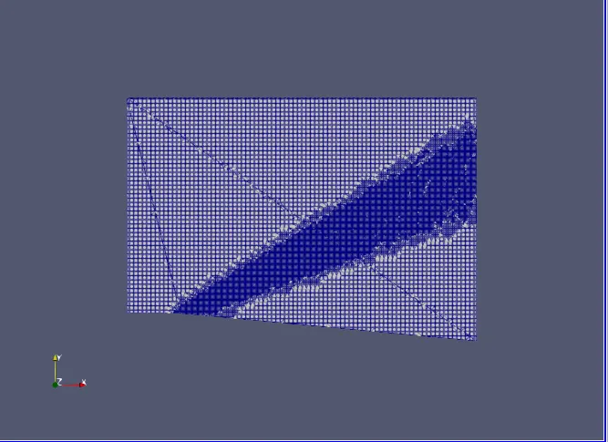
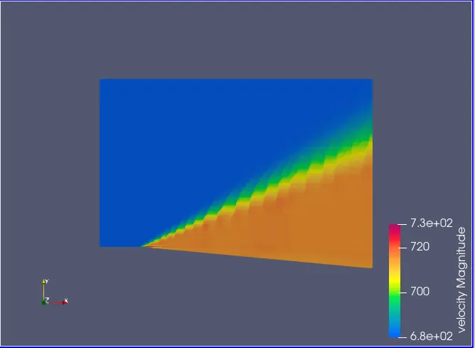
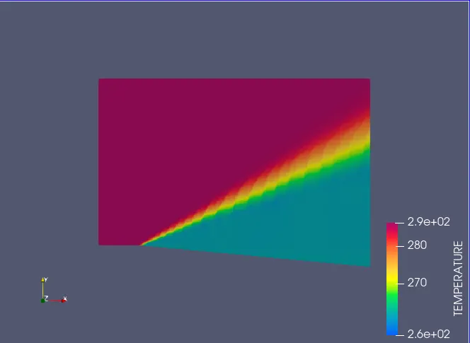
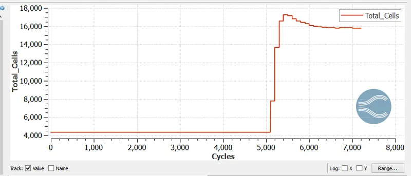
case 2-when SGS scale is 0.05
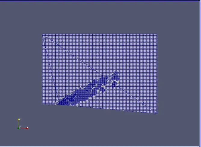
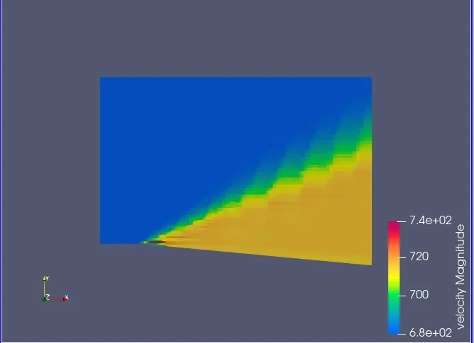
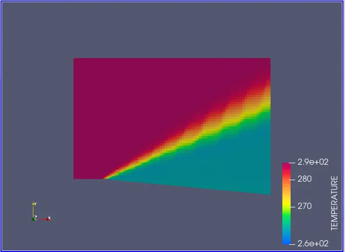
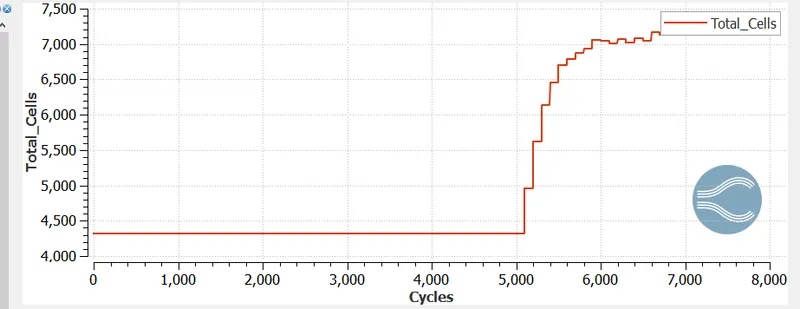
case 3 - when SGS scale is 0.1
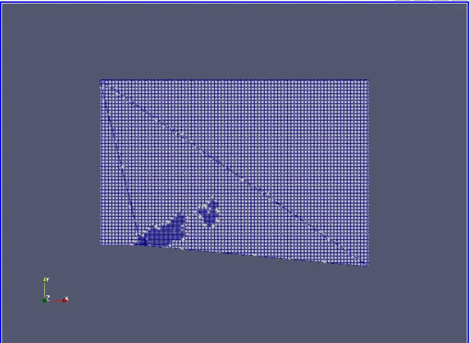
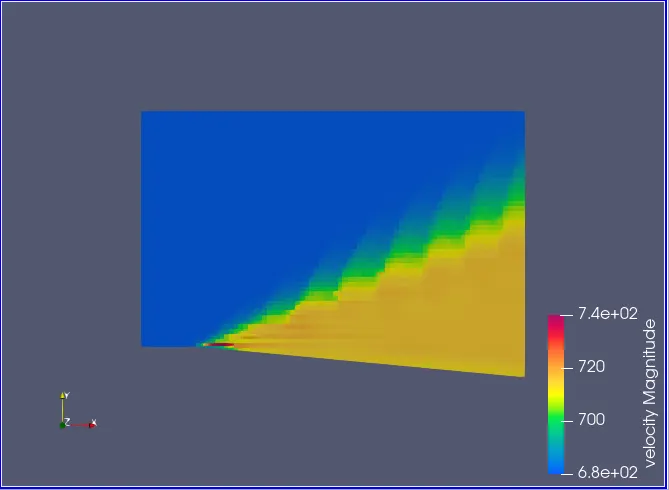
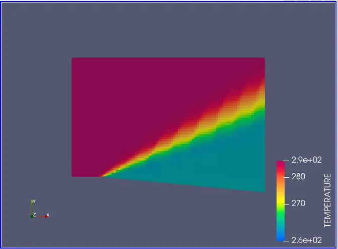
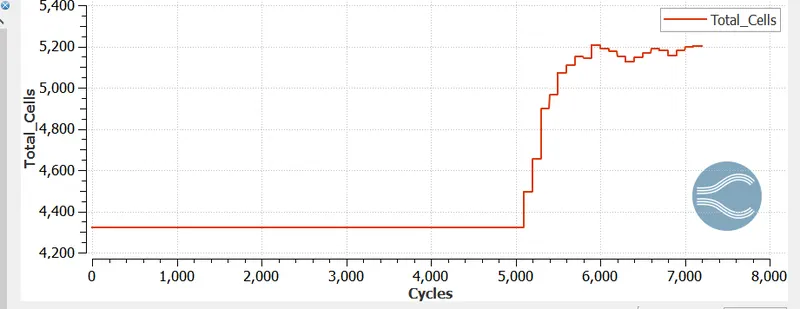
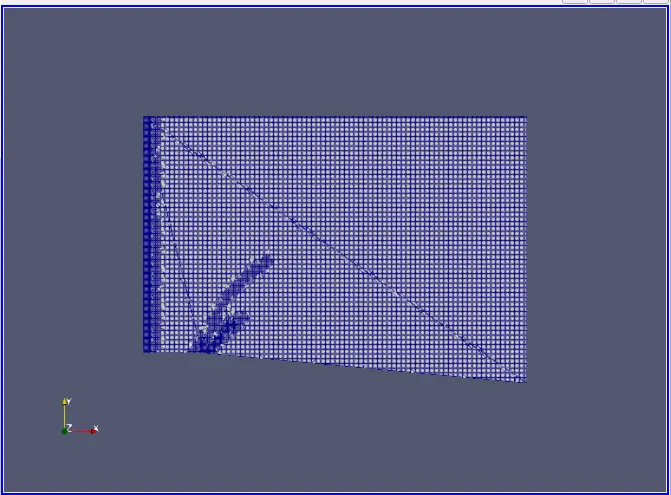
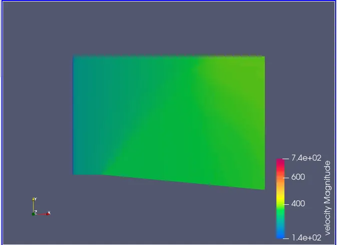
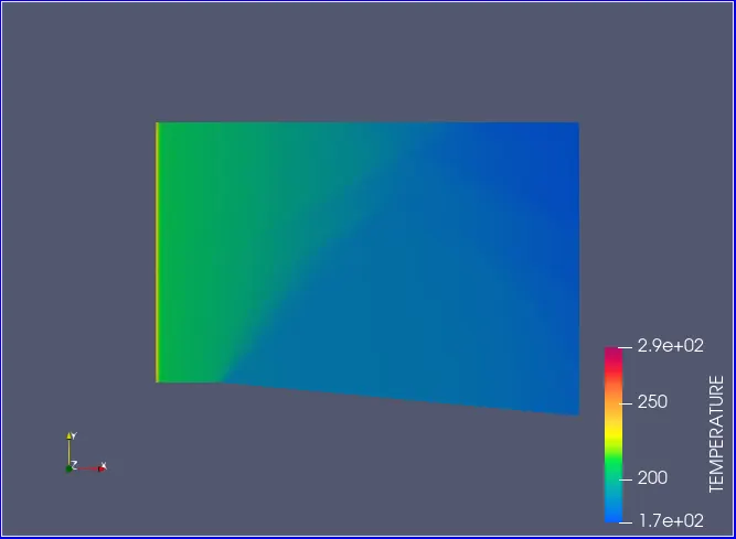
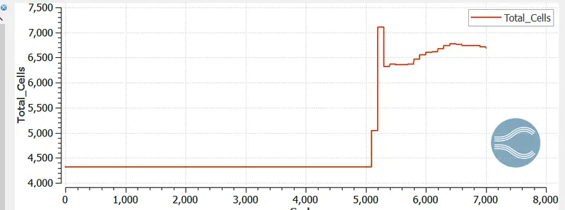
Csae =4 for subsonic for SGS 0.05
conclusion-
1.At SGS of 0.01 the cell count were 17500 and there is large area of refinement around the shock waves.
2.At SGS of 0.05 the cell count were 7500 and we can see that the refinement area around the shock waves is liitle bit narrow than the first case.
3.At SGS of 0.1 the cell count were 5400 and refinement area around the shock waves is very small compared to above two cases .
Hence from above three cases we can conclude that as SGS scale decreases the cell count are going to increases and the refinement area around the shock waves is going to be broad.and for subsonic flow we can see that there no exapnsion.
co
sa
sa