Week 3 - Taylor table method and Matlab code

The Taylor table for skewed for right hand side is given as

f(x) f'(x) f"(x)^2 f"'(x)^3 f"''(x)^4 f""'(x)^5

aF(i) a 0 0 0 o 0.

bF(i+1) b b b/2 b/6 b_/24 b/125

cF(i+2) c 2c 4c/2 8c/6 16c/24 32d/125

dF(i+3) d 3d 9d/2 27d/6 81d/24 243d/125

e F(i+4) e 4e 16e/2 56d/6 256e/24 1024e/125

f F(i+5) f 5f 25f/2 125f/6 625f/24 3125f/125

from above table we can write as

f(i)=af(x)..(1)

bf(i+1)=bf(x) +b* f'(x) +b*f''(x) *x^2/2+bf'''(x)*x^3/6+bf''''(x)*x^4/24+bf'''''(x)*(x)^5...(2)

cf(i+2)=cf(x) +c* f'(x) 2*x +c*f''(x) *4(x^2)/2+cf'''(x)*8(x^3)/6+bf''''(x)*(16)x^4/24+bf'''''(x)32*(x)^5...(3)

df(i+3)=df(x) +d* f'(x) 3*x +d*f''(x) *9(x^2)/2+df'''(x)*27(x^3)/6+df''''(x)*(81)x^4/24+df'''''(x)243*(x)^5...(4)

ef(i+4)=ef(x) +e* f'(x) 4*x +e*f''(x) *16(x^2)/2+ef'''(x)*64(x^3)/6+ef''''(x)*(256)x^4/24+ef'''''(x)1024*(x)^5...(5)

f(i+5)=f*f(x) +f* f'(x) 5*x +f*f''(x) *25(x^2)/2+f*f'''(x)*125(x^3)/6+f*f''''(x)*(625)x^4/24+f*f'''''(x)3125*(x)^5....(6) since we have six equation and six unknowns hence by matlab we can find values of coeefiicents

q=[1,1,1,1,1,1;0,1,2,3,4,5;0,1/2,4/2,9/2,16/2,25/2;0,1/6,8/6,27/6,64/6,125/6;0,1/24,16/24,81/24,256/24,625/24;0,1/120,32/120,243/120,1024/120,3125/120]
p=[0;0;1;0;0;0]
x=rats(linsolve(q,p))

and we get values as

 '     15/4     '
    '    -77/6     '
    '    107/6     '
    '      -13     '
    '     61/12    '
    '     -5/6     '

and adding eqqns(1)+(2)+(3)+(4)+(5)+(6)

we get

af(i)+bf(i+1)+cf(i+2)+cf(i+3)+ef(i+4)+f*f(i+5)=f(x)(a+b+c+d+e+f)+f'(x)/(0a+b+2c+3d+4e+5f)+f''(x)/2*(0a+1b+4c+9d+16e+25f)+f'''(x)/6*(0a+1b+8c+27d+56e+125f)+f''''(x)/24(0a+1b+16c+81d+256e+625f)+f'''''(x)/125(0a+1b+32c+243d+1024e+3125f)

since the sum of f'(x),f(x),f''(x) and f'''(x)=0 we left with

af(i)+bf(i+1)+cf(i+2)+cf(i+3)+ef(i+4)+f*f(i+5)=f''(x)/2*(0a+1b+4c+9d+16e+25f)+f'''''(x)/125(0a+1b+32c+243d+1024e+3125f)

but on substituing values of a.b,c,d,e,f we getf''''(x)*x^5=0

hence we left with

af(i)+bf(i+1)+cf(i+2)+cf(i+3)+ef(i+4)+f*f(i+5)=f''(x)*x^2/2*(0a+1b+4c+9d+16e+25f)

divding lhs and rhs by x^2 and substituing valyes of a,b,c,d,e,f

af(i)+bf(i+1)+cf(i+2)+cf(i+3)+ef(i+4)+f*f(i+5)/x^2=f''(x) simillarly tabl e for skewd left

	f(i)	f'(x)	f'''(x)^2	f'''(x)^3	f(x)'''(x)^4	f(x)''''(x)^5
f(i)	a	o	o	0	o	0
f(i-1)	b	-b	b/2	-b/6	b\24	-b/125
f(i-2)	c	-2c	c4/2	-8c/6	16c/24	-32c/125
f(i-3)	d	-3d	d9/2	-27d/6	81d/24	-243d/125
f(i-4)	e	-4e	16e/2	-64e/6	256e/24	-1024e/125
f(i-5)	f	-5f	25f/2	-125/6	625f/24	-3125f/125-

f(i)=af(x)..(1)

bf(i-1)=bf(x) -b* f'(x) +b*f''(x) *x^2/2-bf'''(x)*x^3/6+bf''''(x)*x^4/24-bf'''''(x)*(x)^5...(2)

cf(i-2)=cf(x) -c* f'(x) 2*x +c*f''(x) *4(x^2)/2-cf'''(x)*8(x^3)/6+bf''''(x)*(16)x^4/24-bf'''''(x)32*(x)^5...(3)

df(i-3)=df(x) -d* f'(x) 3*x +d*f''(x) *9(x^2)/2-df'''(x)*27(x^3)/6+df''''(x)*(81)x^4/24-df'''''(x)243*(x)^5...(4)

ef(i-4)=ef(x) -e* f'(x) 4*x +e*f''(x) *16(x^2)/2-ef'''(x)*64(x^3)/6+ef''''(x)*(256)x^4/24-ef'''''(x)1024*(x)^5...(5)

f(i-5)=f*f(x) -* f'(x) 5*x +f*f''(x) *25(x^2)/2-f*f'''(x)*125(x^3)/6+f*f''''(x)*(625)x^4/24-f*f'''''(x)3125*(x)^5....(6)

r=[1,1,1,1,1,1;0,-1,-2,-3,-4,-5;0,1/2,4/2,9/2,16/2,25/2;0,-1/6,-8/6,-27/6,-64/6,-125/6;0,1/24,16/24,81/24,256/24,625/24;0,-1/120,-32/120,-243/120,-1024/120,-3125/120]
s=[0;0;1;0;0;0]
t=rats(linsolve(r,s))

and the value of coefficients are

 '     15/4     '
    '    -77/6     '
    '    107/6     '
    '      -13     '
    '     61/12    '
    '     -5/6     '

af(i)+bf(i-1)+cf(i-2)+cf(i-3)+ef(i-4)+f*f(i-5)=f''(x)*x^2/2*(0a+1b+4c+9d+16e+25f)

divding lhs and rhs by x^2 and substituing valyes of a,b,c,d,e,f

af(i)+bf(i-1)+cf(i-2)+cf(i-3)+ef(i-4)+f*f(i-5)/x^2=f''(x)

taylor table for central difference

	f(i)	f'(i)x	f''(i)x^2	f'''(i)x^3	f''''(i)x^4
f(i-2)	a	-2a	4a/2	-8a/6	16a/24
f(i-1)	b	-b	b/2	-b/6	b/24
f(x)	c	0	0	0	0
f(i+1)	d	d	d/2	d/6	d/24
f(i+2)	e	2e	4e/2	8e/6	16e/24
sum of columns	0	0	1	0	0

f(i-2)=af(x) -a* f'(x) 2*x +a*f''(x) *4(x^2)/2-af'''(x)*8(x^3)/6+af''''(x)*(16)x^4/24-af'''''(x)32*(x)^5

bf(i-1)=bf(x) -b* f'(x) +b*f''(x) *x^2/2-bf'''(x)*x^3/6+bf''''(x)*x^4/24-bf'''''(x)*(x)^5

f(i)=cf(x)

df(i+1)=df(x) +d* f'(x) +d*f''(x) *x^2/2+df'''(x)*x^3/6+df''''(x)*x^4/24+df'''''(x)*(x)^5

.e(i+2)=ef(x) +e* f'(x) 2*x +e*f''(x) *4(x^2)/2+ef'''(x)*8(x^3)/6+ef''''(x)*(16)x^4/24+ef'''''(x)32*(x)^5.

sice we have 5 equation and 5 unknowns

a=[1,1,1,1,1;-2,-1,0,1,2;4/2,1/2,0,1/2,4/2;-8/6,-1/6,0,1/6,8/6;16/24,1/24,0,1/24,16/24]
b=[0;0;;1;0;0]
c=rats(linsolve(a,b))

the value of the coeeficients are

 -1/12    '
    '      4/3     '
    '     -5/2     '
    '      4/3     '
    '     -1/12    '

after adiind 1,2,3,4,5 and subjusting the values of a,b,c,d,e we get

af(i-2)+bf(i-1)+cf(i)+df(i)+ef(i+1)+ef(i+2)/x^2=f''(x)

and let us apply above producer fror van function

exp(x)*cos(x)

and the code is as follows

x=pi/3
dx=linspace(pi/4,pi/400,50)

analytical_solution=-2*exp(x)*sin(x)
for i=1:length(dx)
   skewed_right_side=((15/4)*((exp(x)*cos(x)))-(77/6)*((exp(x+(1.*dx)).*cos(x+(1.*dx))))+(107/6)*((exp(x+(2.*dx)).*cos(x+(2.*dx))))-13*((exp(x+(3.*dx)).*cos(x+(3.*dx))))+(61/12)*((exp(x+(4.*dx)).*cos(x+(4.*dx))))-(5/6)*((exp(x+(5.*dx)).*cos(x+(5.*dx)))))./(dx.^2)
    skewed_left_side=((15/4)*((exp(x)*cos(x)))-(77/6)*((exp(x-(1.*dx)).*cos(x-(1.*dx))))+(107/6)*((exp(x-(2.*dx)).*cos(x-(2.*dx))))-13*((exp(x-(3.*dx)).*cos(x-(3.*dx))))+(61/12)*((exp(x-(4.*dx)).*cos(x-(4.*dx))))-(5/6)*((exp(x-(5.*dx)).*cos(x-(5.*dx)))))./(dx.^2)
    central_difference=(-(1/12)*((exp(x-(2.*dx)).*cos(x-(2.*dx))))+(4/3)*((exp(x-(1.*dx)).*cos(x-(1.*dx))))-(5/2)*((exp(x)*cos(x)))+(4/3)*((exp(x+(1.*dx)).*cos(x+(1.*dx))))-(1/12)*((exp(x+(2.*dx)).*cos(x+(2.*dx)))))./(dx.^2)
    
    out=abs(skewed_right_side-analytical_solution)
    out_2=abs(skewed_left_side-analytical_solution)
    out_3=abs(central_difference-analytical_solution)
end

loglog(dx,out,'r','linewidth',2)
hold on
loglog(dx,out_2,'b','linewidth',2)
hold on
loglog(dx,out_3,'g','linewidth',2)
grid on
xlabel('dx')
ylabel('error')
legend('skewed-right','skewed-left','central-difference')
    
    

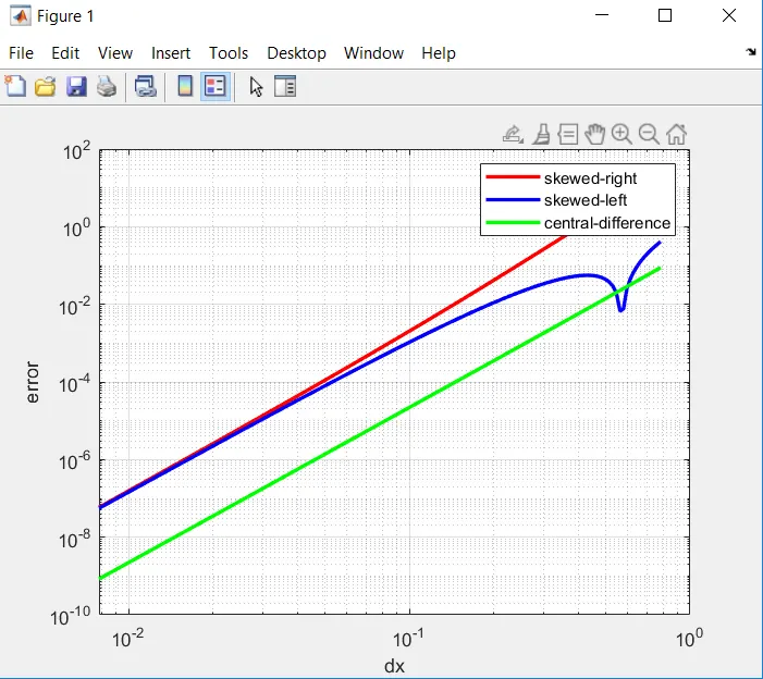
observation

From the graph we observe that as the grid size increases the error value increases for the skewed-right,left the error is less becuse the number of terms are more i.e (4+2) where 4 is the degree of apporximations and 2 is the order of the differtential equation and for the central difference the error is more because the number of terms are less i.e (4+2-1).

why we need skeweness distrubution

skewness uses the data values at the points from right side or from left side but central difference use the data values from the both right and left side of the nodes which is symmmentry ,and skeweness deviate the symmentry and skewness results less error becuse it uses more terms and central difference uses less terms than the skewness.