Week 4 - Genetic Algorithm

Theroy;-

Genetic algorthim is method of finding the optimum solution for the objective function subjected to the both constrained and unconstrained.genetic algorthim is widely used in machine learning and in artifical intellegience to slove the complex poroblems like travell space problems and the expotential ptoblems.

The main steps in genetic algorthim are

1. Intial population- its an array consting of the exsiting solution for the objective function .the main point in the intial population is diversity as the diversity increases we get the more optimum solution for the function.

2. calculate fitness- fitness is the most revelant output to the input.its calculated by comparing the output with an array of the intial population for an example if we an input array as 'TAKE',and we have the output as 'FAKE', by comparing the output with an input we have fitness value as 3. if we have an output has 'AEBC', by comparing we have the fitness value has 1.

3.selection- selection is directly proptional to the fitness value.we are selecting the parents whose fitness value is greater than the other values,for producing the next generation.

4.crossover-its method of producing the next generation from the parential solution.the crossover should be such that fitness value the new generation should be different from the fitness value of the intial population array. and they are various method in crossover such as onepoint,multi point method.

5.mutation- its the method of bringing the changes in the offsprings. they are various methods in mutation such as swap,flip method.

producer-

1.The sepertae stagalmite function is written in different script file.

2.the x and the y values are extraxcted from the input _vector

3.the negative sign used becuse to get maximum function.

function[ f]=stagalmite3(input_vector)
x=input_vector(1);
y=input_vector(2);
f1=(sin(5*pi*x+0.5)).^6;
f2=exp(-4*log(2)*((x-0.0667).^2)./0.64);
f3=(sin(5*pi*y+0.5)).^6;
f4=exp(-4*log(2)*((y-0.0667).^2)./0.64);
f=-(f1*f2*f3*f4);
end

4.the x and the y values are created using the linspace commannd bewtten 0 and 0.6

5. the one dimensional array is converted in to two dimensional using the mesh grid option.

6.the nested for loop is used because to iterate the calculation of the value of the function up to lengths of the x and the y values.

7.the variable input_vector(1) is used to store the values of xx and input_vector(2) to store the values of the yy.

8.after the calculation of the value of the function for different values of x and y the calculated values are stored in the variable called F which is 150*150.

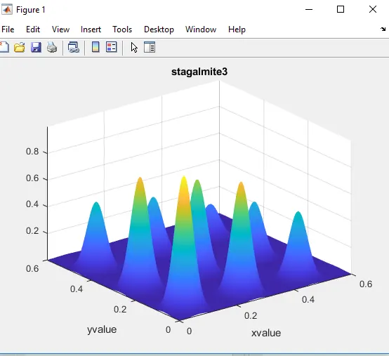
9.the surfc command is used to convert the three dimesional image the general syntax for surfcis (x,y,z) but in this problem we want the three dimensional of (xx,yy,-F)

x=linspace(0,0.6,150)
y=linspace(0,0.6,150)
[xx yy]=meshgrid(x,y)
for i= 1:length(xx)
    for j=1:length(yy)
        input_vector(1)=xx(i,j);
        input_vector(2)=yy(i,j);
        F(i,j)=stagalmite3(input_vector);
    end
end
surfc(xx,yy,-F);
shading interp

xlabel('xvalue')
ylabel('yvalue')
title('stagalmite3')

10. The main objective is used to find the optimum solution form the array of the intial poplation of the solution of the function i.e from the arry of F.

11.For this we use the genetic algaorthim the general syntax is x=ga(@function,number of variables)

where is the function is the name of the function here in this problem we use the function called stagalmite and here is the number of variables is 2 i.e x and y.

12.in this problem we have used for loop to calculate optmium values for the function for 50 times and [inputs,Fopt(i)]=ga(@tagalmite,2) the output variable 'inputs 'is used to store the value of x and y for which the function will be optimum.and the size of the inputs 1*2 which is going to store the value of xand y for each iteration.and the output variable Fopt(i)is used to store the values of optmium values of trhe function which size of 1*50.

13.The xopt(i) is used to store the values of x at which the function is optimum and yopt(i) is used to store the values of y at which the function will be optimum. and the size of xopt(i) and yopt(i) is 1*50 becuse we are going to iterate for 50 times.

14. we have used the command called subplot and the bsyntax for subplot is(m,n,p) it divides the window in to m by n matrix and p gives current position of the plot.here in this problem we have usedsubplot(2,1,1) means the window is divided in to 2 rows and one column and p=1 the first plot is in (1,1).

15.we have used command called surfc to create three dimensional image of the (x,y,-f)

16.we have used plot command to plot the values of xopt,yopt anf -Fopt .

17.we have used another subplot to plot the -Fopt vlues for different iteration. which lies in (2,1) hence we have used subplot(2,1,2).

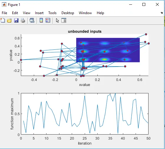
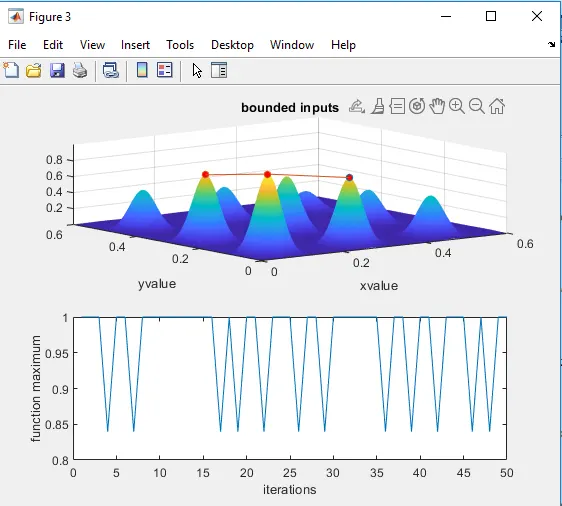
18.the main drawbrack of the above method is ga takes the values of x and y below zero and greater than 0.6 to calculate the fopt value.hence in order to

aviod this drawback we upper bound limit and the lower bound limit for both x and y values.nad the syntax for that is given has [inputs,fval]=ga(@function,no.of variables,A,b,Aeq.beq,upper bound limit,lower bound limit)

what are (A,b,Aeq.beq, are explained by connsidering the example)

we use the A,b when the function is subjected to linear inequality constraint for eg

x1+2x2-4x3<12-(1)

2x1-3x3<11-(2)

the eqn(1,2)resprents linear inequality constriants hence A is written has A=[1,2,-4;2,0,-3] abd b=[12;11]

we use thye Aequn and beqn used when function is subjected to linear equality constraints

for eg

x1+2x2-4x3=12-(3)

2x1-3x3=11-(4)

the eqn(3,4)respernt linear equality constraints and Aeqn =[1,2,-4;2,0,-3] and beqn=[12;11]

19.for this example i.e stagalmite function is not subjected to any constraints hence we use A,b,Aeqn,beqn as null vectors

and the code is as follows

tic
for i=1:num_cases
    [inputs,fopt(i)]=ga(@stagalmite3,2,[],[],[],[],[0;0],[0.6;0.6])
     
    xopt(i)=inputs(1)
    yopt(i)=inputs(2)
end
study_time2=toc
figure(3)
subplot(2,1,1)


surfc(x,y,-f)
shading interp
title('bounded inputs')
xlabel('xvalue')
ylabel('yvalue')
hold on
plot3(xopt,yopt,-fopt,'marker','o','markersize',5,'markerfacecolor','r')
subplot(2,1,2)
plot(-fopt)
xlabel('iterations')
ylabel('function maximum')

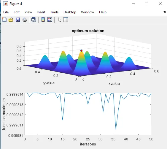
20. our main objective is used to find global solution for the function as in early method we limited number of option i.e 50,hence we have an local maxima in order to have global solution we increase the population size for that we use the option command which generates more option for the optimmisation.and the code is follows

options=optimoptions(@ga)
options=optimoptions(options,'populationsize',170)
tic
for i=1:num_cases
[inputs fopt(i)]=ga(@stagalmite3,2,[],[],[],[],[0;0],[0.6;.6],[],[],options)
xopt(i)=inputs(1)
yopt(i)=inputs(2)
end
study_time3=toc
figure(4)
subplot(2,1,1)


surfc(x,y,-f)
shading interp
title('optimum solution')
xlabel('xvalue')
ylabel('yvalue')
hold on
plot3(xopt,yopt,-fopt,'marker','o','markersize',5,'markerfacecolor','r')
subplot(2,1,2)
plot(-fopt)
xlabel('iterations')
ylabel('function maximum')