Week 5.1 - Mid term project - Solving the steady and unsteady 2D heat conduction problem
we have 2d heat conduction as
(dT/dx)^2+(dt/dy)^2=0...(1)
we apply central difference for the eq(1) as
(T(i-1,j)-2T(i,j)+T(i+1,J)/(dx)^2)+(T(i,j-1)-2T(i,j)+T(i,j+1))/(dy)^2)=0
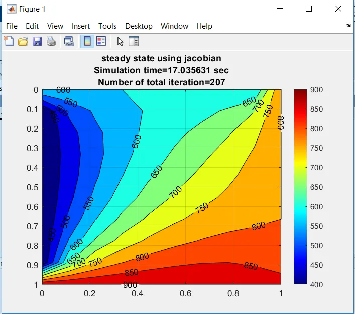
we have code for the jacobian steady state as
l=1;
nx=10;
ny=10;
x=linspace(0,l,nx);
dx=x(2)-x(1);
y=linspace(0,l,ny);
dy=y(2)-y(1);
T=300*ones(nx,ny);
T(:,1)=400;
T(1,:)=600;

T(:,end)=800;

T(end,:)=900;
T_old=T;
term=(dx^2*dy^2)/(2*(dx^2+dy^2));
tol=1e-4;
error=1;
iteration_method=1;
if iteration_method==1;
    tic;
    iter_num=0;
    while(error>tol)
       for j=2:ny-1
           for i=2:nx-1
             TL=T_old(i-1,j)
               TR=T_old(i+1,j)
               TB=T_old(i,j-1)
               TT=T_old(i,j+1)
               H=(TL+TR)/(dx^2)
               V=(TB+TT)/(dy^2)
               T(i,j)=term*(H+V)

           end
       end


        error=max(max(abs(T-T_old)));
        T_old=T;
        iter_num=iter_num+1;
    end
    cal_time=toc;

end
[x,y]=contourf(x,y,T)
clabel(x,y)
colorbar
colormap(jet)
ax=gca
ax.YDir='reverse'
title_text1=sprintf('Simulation time=%f sec',cal_time)
title_text2=sprintf('Number of total iteration=%d',iter_num)
title({'steady state using jacobian';title_text1;title_text2})
grid on
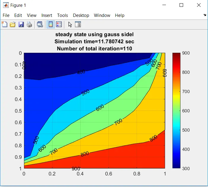
we have code for gauss sidel method
l=1
nx=10
ny=10;
x=linspace(0,l,nx)
dx=x(2)-x(1)
y=linspace(0,l,ny)
dy=y(2)-y(1)
T=300*ones(nx,ny)
T(:,1)=400

TT(1,:)=600
T(:,end)=800
T(end,:)=900
T_old=T;
term=(dx^2*dy^2)/(2*(dx^2+dy^2));
tol=1e-4;
error=1;
iteration_method=2
if iteration_method==2
    tic

    iter_num=0

while(error>tol)


       for j=2:ny-1
           for i=2:nx-1

             TL=T(i-1,j)
               TR=T_old(i+1,j)
               TB=T(i,j-1)
               TT=T_old(i,j+1)
               H=(TL+TR)/(dx^2)
               V=(TB+TT)/(dy^2)
               T(i,j)=term*(H+V)

           end
       end


         error=max(max(abs(T-T_old)))
          T_old=T
         iter_num=iter_num+1
end
    cal_time=toc
end

[x,y]=contourf(x,y,T)
clabel(x,y)
colorbar
colormap(jet)
ax=gca
ax.YDir='reverse'
title_text1=sprintf('Simulation time=%f sec',cal_time)
title_text2=sprintf('Number of total iteration=%d',iter_num)
title({'steady state using gauss sidel';title_text1;title_text2})
grid on
the code for the sor method is given as
l=1
nx=10
ny=10;
x=linspace(0,l,nx)
dx=x(2)-x(1)
y=linspace(0,l,ny)
dy=y(2)-y(1)
T=300*ones(nx,ny)
T(:,1)=400

TT(1,:)=600
T(:,end)=800
T(end,:)=900
T_old=T;
term=(dx^2*dy^2)/(2*(dx^2+dy^2));
tol=1e-4;
error=1;
iteration_method=2
if iteration_method==2
    omega=1.8
    tic

    iter_num=0

while(error>tol)


       for j=2:ny-1
           for i=2:nx-1

             TL=T(i-1,j)
               TR=T_old(i+1,j)
               TB=T(i,j-1)
               TT=T_old(i,j+1)
               H=(TL+TR)/(dx^2)
               V=(TB+TT)/(dy^2)
               T(i,j)=term*(H+V)
               T(i,j)=T_old(i,j)*(1-omega)+(omega*T(i,j))

           end
       end


         error=max(max(abs(T-T_old)))
          T_old=T
         iter_num=iter_num+1
end
    cal_time=toc
end

[x,y]=contourf(x,y,T)
clabel(x,y)
colorbar
colormap(jet)
ax=gca
ax.YDir='reverse'
title_text1=sprintf('Simulation time=%f sec',cal_time)
title_text2=sprintf('Number of total iteration=%d',iter_num)
title({'steady state using sor';title_text1;title_text2})
grid on
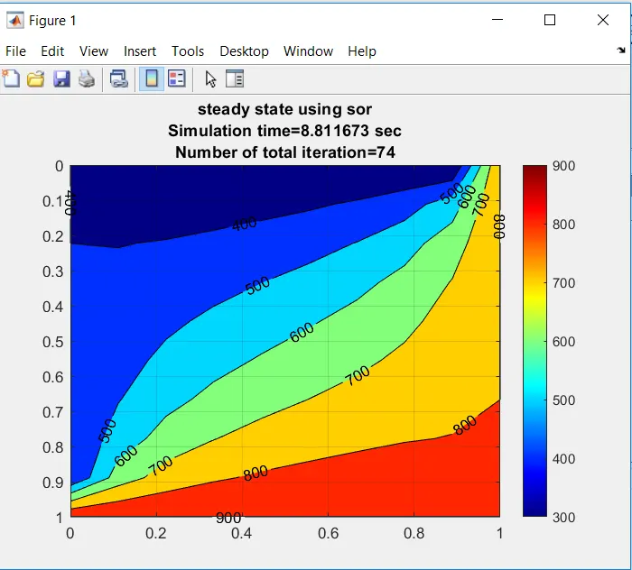
| sl.no | methods | iterations | simulation time(sec) | number of grid points (nx,ny) |
| 1 | Jacobian | 207 | 17.20 | (10,10) |
| 2 | Gauss Sidel | 110 | 11.780 | (10,10) |
| 3 | Sor | 74 | 8.811 | (10,10) |
1.first we create the array fot the x and yby using the command linspace which creates the elements of array bewteen 0 to the 1 up to the length of n.
2.we have used T=300*(1,n) meaning its going to print the row elements up to length of n and the elements are of 1
if we want the elements of the row as zero then we can write as u=zero(1,5) here n=5 then its going to print as 0 0 0 0 0 .
3.the dx is calculated as x(i+1)-x(i) the dx will be same as there is equal spacing.
4.now we define the boundary condtion at the top and the bottom as
Top Boundary = 600 K
Bottom Boundary = 900 K
Left Boundary = 400 K
Right Boundary = 800 K
5.we have used another for loop to calculate the velocity which is given asT(i,j)=term*(T_old(i-1,j)+T_old(i+1,j)+T_old(i,j-1)+T_old(i,j+1)) at different node of discretization.when we simulate for some time the velocity is going to change from intial velocity hence that change in velocity is going to store in T_oldand for next simultion previous velocity wich is stored in T_old is used to calcULATE.
6.same method is uded for gauss sidel olny change in the eqn T(i,j)=term(T(i-1,j)+T_old(i+1,j)+T(i,j-1)+T_old(i,j+1))here we are uing upgated T values for T(i-1,j) since we have for (i-1) and we use old value for the (i+1) since we dont have upgated value for the (i+1),same applicable for column element.
Now we apply jacobi,gauss sidel and sir fir explict function
For explict we have 2d heat conduction as
d^2T/dt^2=alpha*((d^2T/dx^2)+(d^2T/dy^2))
We apply forward differencing for time and central differencing for the space dervative we get as
T^n+1-T^n=alpa*((T(I-1,j)-2T(I,j)+T(i+1,j)/dx^2)+T(I,j-1-2T(i,j)+T(i,j+1)/dy^2)...(2)
Eq(2) can be written as
T(i j)^(n+1)=T^n(i j)+(k1*(T(I-1,j)+T(i+1,j)^(n+1))+(k2*((T(i,j-1)+T(i,j+1)^(n+1))
Where k1=alpha/dx^2 and k2=apla/dy^2
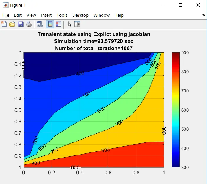
the code for the jacobian slover
l=1;
nx=10
ny=10;
dt=10
t=1000
nt=t/dt
alpa=1.75e-4
x=linspace(0,l,nx)
dx=x(2)-x(1)
y=linspace(0,l,ny)
dy=y(2)-y(1)
CFL=alpa*dt*((1/dx^2)+(1/dy^2))
T=300*ones(nx,ny)
T(:,1)=400

TT(1,:)=600
T(:,end)=800
T(end,:)=900
T_old=T;
T_prev=T
k1=alpa*dt/dx^2
k2=alpa*dt/dy^2
term=(dx^2*dy^2)/(2*(dx^2+dy^2));
tol=1e-4;
error=1;
iteration_method=1
if iteration_method==1
    tic

    iter_num=0
    for k=1:nt
      error=1
while(error>tol)


       for j=2:ny-1
           for i=2:nx-1
            term1=1/(1+2*k1+2*k2)
            term2=k1*term1
            term3=k2*term1
             TL=T_old(i-1,j)
               TR=T_old(i+1,j)
               TB=T_old(i,j-1)
               TT=T_old(i,j+1)
               H=(TL+TR)
               V=(TB+TT)
               T(i,j)=(T_prev(i,j)*term1)+(H*term2)+(V*term3)

           end
       end


         error=max(max(abs(T-T_old)))
          T_old=T
         iter_num=iter_num+1
end
T_prev=T
    end


    cal_time=toc
end

[x,y]=contourf(x,y,T)
clabel(x,y)
colorbar
colormap(jet)
ax=gca
ax.YDir='reverse'
title_text1=sprintf('Simulation time=%f sec',cal_time)
title_text2=sprintf('Number of total iteration=%d',iter_num)
title({'Transient state using Explict using jacobin';title_text1;title_text2})
grid on
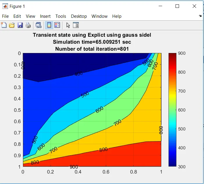
The code for Explict gauss sidel
l=1
nx=10
ny=10;
dt=10
t=1000
nt=t/dt
alpa=1.75e-4
x=linspace(0,l,nx)
dx=x(2)-x(1)
y=linspace(0,l,ny)
dy=y(2)-y(1)
CFL=alpa*dt*((1/dx^2)+(1/dy^2))
T=300*ones(nx,ny)
T(:,1)=400

TT(1,:)=600
T(:,end)=800
T(end,:)=900
T_old=T;
T_prev=T
k1=alpa*dt/dx^2
k2=alpa*dt/dy^2

tol=1e-4;

iteration_method=2
if iteration_method==2
    tic

    iter_num=1
    for k=1:nt
      error=4e4
while(error>tol)


       for j=2:ny-1
           for i=2:nx-1
            term1=1/(1+2*k1+2*k2)
            term2=k1*term1
            term3=k2*term1
             H=(T(i-1,j)+T_old(i+1,j))
             V=(T(i,j-1)+T_old(i,j+1))
               T(i,j)=(T_prev(i,j)*term1)+(H*term2)+(V*term3)

           end
       end


         error=max(max(abs(T-T_old)))
          T_old=T
         iter_num=iter_num+1
end
T_prev=T
    end


    cal_time=toc
end

[x,y]=contourf(x,y,T)
clabel(x,y)
colorbar
colormap(jet)
ax=gca
ax.YDir='reverse'
title_text1=sprintf('Simulation time=%f sec',cal_time)
title_text2=sprintf('Number of total iteration=%d',iter_num)
title({'Transient state using Explict using gauss sidel';title_text1;title_text2})
grid on
the code for Explict Sor method
l=1

nx=10

ny=10;

dt=10

t=1000

nt=t/dt

alpa=1.75e-4

x=linspace(0,l,nx)

dx=x(2)-x(1)

y=linspace(0,l,ny)

dy=y(2)-y(1)

CFL=alpa*dt*((1/dx^2)+(1/dy^2))

T=300*ones(nx,ny)

T(:,1)=400


TT(1,:)=600

T(:,end)=800

T(end,:)=900

T_old=T;

T_prev=T

k1=alpa*dt/dx^2

k2=alpa*dt/dy^2


tol=1e-4;


iteration_method=3

if iteration_method==3

    omega=1.8

    tic


    iter_num=1

    for k=1:nt

      error=4e4

while(error>tol)


       for j=2:ny-1

           for i=2:nx-1

            term1=1/(1+2*k1+2*k2)

            term2=k1*term1

            term3=k2*term1

             H=(T(i-1,j)+T_old(i+1,j))

             V=(T(i,j-1)+T_old(i,j+1))

               T(i,j)=(T_prev(i,j)*term1)+(H*term2)+(V*term3)

               T(i,j)=T_old(i,j)*(1-omega)+(omega*T(i,j))

           end

       end


         error=max(max(abs(T-T_old)))

          T_old=T

         iter_num=iter_num+1

end

T_prev=T

    end


    cal_time=toc

end


[x,y]=contourf(x,y,T)

clabel(x,y)

colorbar

colormap(jet)

ax=gca

ax.YDir='reverse'

title_text1=sprintf('Simulation time=%f sec',cal_time)

title_text2=sprintf('Number of total iteration=%d',iter_num)

title({'Transient state using Exlict using sor';title_text1;title_text2})

grid on
the plot
| sl.no | Method | simulation time (sec) | number of iterations |
| 1 | Jacobian | 93.579 | 1067 |
| 2 | Gauss sidel | 65.00925 | 801 |
| 3 | Sor | 45.789 | 503 |
For implict we have 2d heat conduction as
d^2T/dt^2=alpha*((d^2T/dx^2)^n+(d^2T/dy^2))^n
We apply forward differencing for time and central differencing for the space dervative we get as
T^n+1-T^n=alpa*((T(I-1,j)-2T(I,j)+T(i+1,j)/dx^2)^(n)+T(I,j-1-2T(i,j)+T(i,j+1)/dy^2)^n...(2)
Eq(2) can be written as
T(i j)^(n)=T^(n+1)(i j)+(k1*(T(I-1,j)+T(i+1,j)^(n))+(k2*((T(i,j-1)+T(i,j+1)^(n))
T(i j)^(n)=T^(n+1)(i j)+(k1*(T(I-1,j)+T(i+1,j)^(n))+(k2*((T(i,j-1)+T(i,j+1)^(n))
Where k1=alpha/dx^2 and k2=apla/dy^2
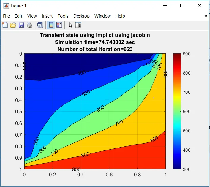
the code for implict jacobian
l=1
nx=10
ny=10;
dt=10
t=1000
nt=t/dt
alpa=1.75e-4
x=linspace(0,l,nx)
dx=x(2)-x(1)
y=linspace(0,l,ny)
dy=y(2)-y(1)
CFL=alpa*dt*((1/dx^2)+(1/dy^2))
T=300*ones(nx,ny)
T(:,1)=400

TT(1,:)=600
T(:,end)=800
T(end,:)=900
T_old=T;
T_prev=T
k1=alpa*dt/dx^2
k2=alpa*dt/dy^2
term=(dx^2*dy^2)/(2*(dx^2+dy^2));
tol=1e-4;
error=1;
iteration_method=2
if iteration_method==2
    tic

    iter_num=0
    for k=1:nt
      error=1
while(error>tol)


       for j=2:ny-1
           for i=2:nx-1
            term1=1/(1+2*k1+2*k2)
            term2=k1*term1
            term3=k2*term1
             TL=T_old(i-1,j)
               TR=T_old(i+1,j)
               TB=T_old(i,j-1)
               TT=T_old(i,j+1)
               H=(TL+TR)
               V=(TB+TT)
               T(i,j)=(T_old (i,j)*term1)+(H*term2)+(V*term3)

           end
       end


         error=max(max(abs(T-T_old)))
          T_old=T
         iter_num=iter_num+1
end

    end


    cal_time=toc
end

[x,y]=contourf(x,y,T)
clabel(x,y)
colorbar
colormap(jet)
ax=gca
ax.YDir='reverse'
title_text1=sprintf('Simulation time=%f sec',cal_time)
title_text2=sprintf('Number of total iteration=%d',iter_num)
title({'Transient state using implict using jacobin';title_text1;title_text2})
grid on
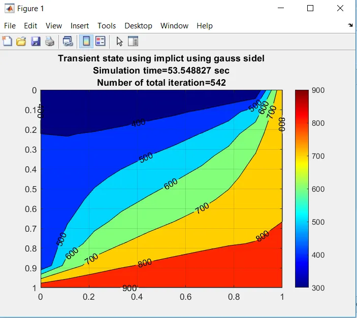
the code for Gauss side
l=1
nx=10
ny=10;
dt=10
t=1000
nt=t/dt
alpa=1.75e-4
x=linspace(0,l,nx)
dx=x(2)-x(1)
y=linspace(0,l,ny)
dy=y(2)-y(1)
CFL=alpa*dt*((1/dx^2)+(1/dy^2))
T=300*ones(nx,ny)
T(:,1)=400

TT(1,:)=600
T(:,end)=800
T(end,:)=900
T_old=T;
T_prev=T
k1=alpa*dt/dx^2
k2=alpa*dt/dy^2

tol=1e-4;

iteration_method=2
if iteration_method==2
    tic

    iter_num=1
    for k=1:nt
      error=4e4
while(error>tol)


       for j=2:ny-1
           for i=2:nx-1
            term1=1/(1+2*k1+2*k2)
            term2=k1*term1
            term3=k2*term1
             H=(T(i-1,j)+T_old(i+1,j))
             V=(T(i,j-1)+T_old(i,j+1))
               T(i,j)=(T_old(i,j)*term1)+(H*term2)+(V*term3)

           end
       end


         error=max(max(abs(T-T_old)))
          T_old=T
         iter_num=iter_num+1
end

    end


    cal_time=toc
end

[x,y]=contourf(x,y,T)
clabel(x,y)
colorbar
colormap(jet)
ax=gca
ax.YDir='reverse'
title_text1=sprintf('Simulation time=%f sec',cal_time)
title_text2=sprintf('Number of total iteration=%d',iter_num)
title({'Transient state using implict using gauss sidel';title_text1;title_text2})
grid on
plot
the code for sor
l=1
nx=10
ny=10;
dt=10
t=1000
nt=t/dt
alpa=1.75e-4
x=linspace(0,l,nx)
dx=x(2)-x(1)
y=linspace(0,l,ny)
dy=y(2)-y(1)
CFL=alpa*dt*((1/dx^2)+(1/dy^2))
T=300*ones(nx,ny)
T(:,1)=400

TT(1,:)=600
T(:,end)=800
T(end,:)=900
T_old=T;
T_prev=T
k1=alpa*dt/dx^2
k2=alpa*dt/dy^2

tol=1e-4;

iteration_method=3
if iteration_method==3
    omega=1.8
    tic

    iter_num=1
    for k=1:nt
      error=4e4
while(error>tol)


       for j=2:ny-1
           for i=2:nx-1
            term1=1/(1+2*k1+2*k2)
            term2=k1*term1
            term3=k2*term1
             H=(T(i-1,j)+T_old(i+1,j))
             V=(T(i,j-1)+T_old(i,j+1))
               T(i,j)=(T_old(i,j)*term1)+(H*term2)+(V*term3)
               T(i,j)=T_old(i,j)*(1-omega)+(omega*T(i,j))
           end
       end


         error=max(max(abs(T-T_old)))
          T_old=T
         iter_num=iter_num+1
end

    end


    cal_time=toc
end

[x,y]=contourf(x,y,T)
clabel(x,y)
colorbar
colormap(jet)
ax=gca
ax.YDir='reverse'
title_text1=sprintf('Simulation time=%f sec',cal_time)
title_text2=sprintf('Number of total iteration=%d',iter_num)
title({'Transient state using implict using sor';title_text1;title_text2})
grid on
the plot
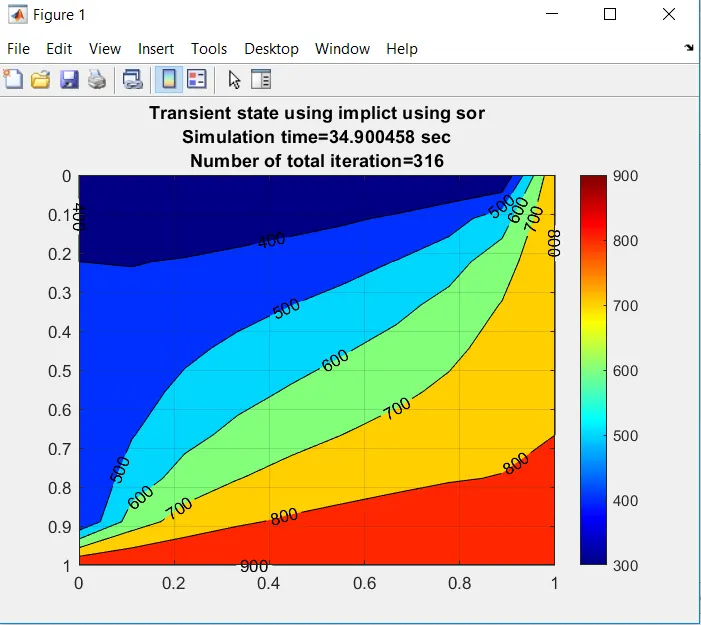
| sl.no | method | simulation | iteraion |
| 1 | jacobian | 74.74 | 623 |
| 2 | Gauss sidel | 53.54 | 542 |
| 3 | Sor | 34.900 | 316 |