Week 5: Prandtl Meyer Shock problem

ABSTRACT:

The following report is a comprehensive description of the phenomnon of expansion fan and the prandtl-meyer function. A CFD simulation is performed for a inlet velocity of 680 m/s over a deflection . The generation of the shock waves is visualized.

Key words- Prandtl_meyer function, Expansion fan, shock waves, MAch number, Converge Studio, PARAVIEW

Objective:

Shock flow boundary conditions

Do a literature search on what BC's are typically used for shock flow problems

2. What is a shock wave?

In your own words, describe the physics behind shock waves

3. Effect of SGS parameter on shock location

In the Prandtl Meyer shock problem, look at the effect of SGS temperature value on cell count and the shock location

Introduction:

This section will cover the theoretical aspects of Prandtl_meyer function, expansion fans and the different boundary conditions used in Shock flow problwms.

Prandtl Meyer Function and expansion fan:

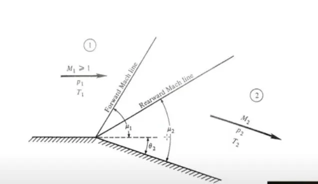
The above image describes the formation of the prandtl-meyer shock waves.

When a supersonic wave encounters a convex corner. the supersonic flow will eventually be turning away from itself, contrary to what happens when it encounters a concave corner. This interaction leads to the formation of expansion waves. Expansion waves are formed when supersonic waves gets away from itself. Unlike a shock, expansion region is continuos, the variation of the properties are relatively smooth. Each line in the expansion fan represents a line of constant properties.

The applications of the Prandtl meyer shock waves are :

• Supersonic vehicles : flow around vehicles, Lift and drag on vehicles.
• Supersonic flow in Nozzles: Flow inside engine nozzles, Thrust produced from nozzles.

Derivation of the Prandtl Meyer Function:

Assumptions:

Isentropic flow.

Contimiuty, momentum conservation and energy conservation equation holds.

Relationships:

• `(dv)/v=-(d(theta))/(M^2-1)^0.5`
• `(dp)/(p)=((gamma*M^2)/((M^2-1))^0.5)*d(theta)`
• `(d(rho))/rho=((M^2/(M^2-1)^0.5)*d(theta)`
• `(dM)/M=(1+(gamma-1)/2*M^2)*(-d(theta))/((M^2-1)^0.5)`

Here , M= mach number , v is the velocity of flow. Rho stands for density , p for pressure.

dtheta is the infinetesimal change in angle by which the flow moves through the convex corner.

The Prandtl meyer function is derived by performing the integration

`nu(M)=((gamma+1)/(gamma-1))^0.5*tan inverse((gamma-1)/(gamma+1)*(M^2-1))^0.5-taninverse(M^2-1)^0.5`

The above equation is called the Prandtl meyer function.

The mach wave angle is given by `mu=sininverse(1/M)`

Boundary conditions:

Boundary conditions (b.c.) are constraints necessary for the solution of a boundary value problem. A boundary value problem is a differential equation (or system of differential equations) to be solved in a domain on whose boundary a set of conditions is known. It is opposed to the “initial value problem”, in which only the conditions on one extreme of the interval are known. Boundary value problems are extremely important as they model a vast amount of phenomena and applications, from solid mechanics to heat transfer, from fluid mechanics to acoustic diffusion. They arise naturally in every problem based on a differential equation to be solved in space, while initial value problems usually refer to problems to be solved in time.

1) Dirichlet Boundary condition:

The Dirichlet boundary condition is a type of boundary condition named after Peter Gustav Lejeune Dirichlet .

In computational fluid mechanics, the classical Dirichlet boundary condition consists of the value of velocity and/or pressure to be taken by a certain set of nodes. It is common to refer to some sets of b.c. according to the following terminology:

• slip boundary condition: the velocity normal to the boundary is set to zero, while the velocity parallel to the boundary is let free
• no-slip boundary condition: both the velocity normal to the boundary and the velocity parallel to the boundary are set equal to zero.

At least one homogeneous b.c. on the pressure (i.e. p=0) has to be imposed as a reference for open domains, for instance, in the highest boundary of the air domain.

2) Neuman Boundary Conditions:

Constraints on the derivative of velocity or pressure fields are mainly used in two cases. The first case is the application of a symmetry plane.

Since this condition is always applied in addition to a Dirichlet b.c. it is naturally satisfied. The second application is the modeling of wall friction, in the case when it is proportional to the strain rate.

Geometry:

The imported file :

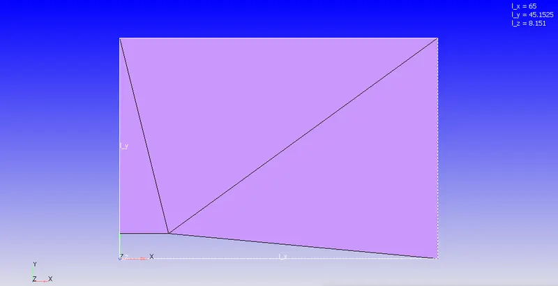
The deflection angle can be found out from the measure-angle option in converge geometry dock. The angle came out to be 5.64 degrees.

The boundary flagging is done like:

• INLET
• OUTLET
• 2D-FRONT
• 2D BACK
• SLIP WALLS

Case set up:

• Application type : Time based

On clicking apply, Converge studio by default loads values for the following groups Gas compressible steady flow.

1) Solver parameters

2) Steady state monitor parameters

3) Simulation time parameters

• Materials :

The pre-defined mixture is selected as Air. Gas simulation box is checked. Species is turned on.

Under the Gas simulation tab, all the pre loaded values are kept un altered. Redlich-Kyong equation of state is used.

The turbulent prandtl and turbulent schimdt number is kept unchanged from the preloaded values.

In the species tab, under gas , The constituents of air, that is O2 and N2 is added .

• Simulation parameters :

Under the Run parameters , New run is opted.

The steady state solver is used for a full hydrodynamic case , The gas flow solver is compressible.

The surface file is loaded from the current geometry surface.dat

In the miscellaneous section, the momentum equation solve is checked. If the shared memory is checked by default, it is unchecked. A steady state monitor is created.

Steady state monitor :

Monitor variables : Mass flow rate

Target type : Boundary

Target : outlet

Monitor start delay : 10000

sample size : 1000

The file in which the values will be stored after the simulation is mass_avg_flow.out

The steady state monitor is the variable that will be monitored through out the simulation. The monitor start delay signifies the value or the number of cycles after which the monitor variable will start being monitored.

Simulation time parameters:

Start time	0
End time	25000
initial time step	1e-9
minimum time step	1e-9
maximum time step	1
maximum CFL convection limit	1
Maximum Diffusion CFL limit	2
Maximum MAch CFL limit	50

Solver parameters :

Density based solver is opted for.

The Navier stokes Solver scheme is PISO

The maximum convection limit is set to 1.

• Boundary conditions:

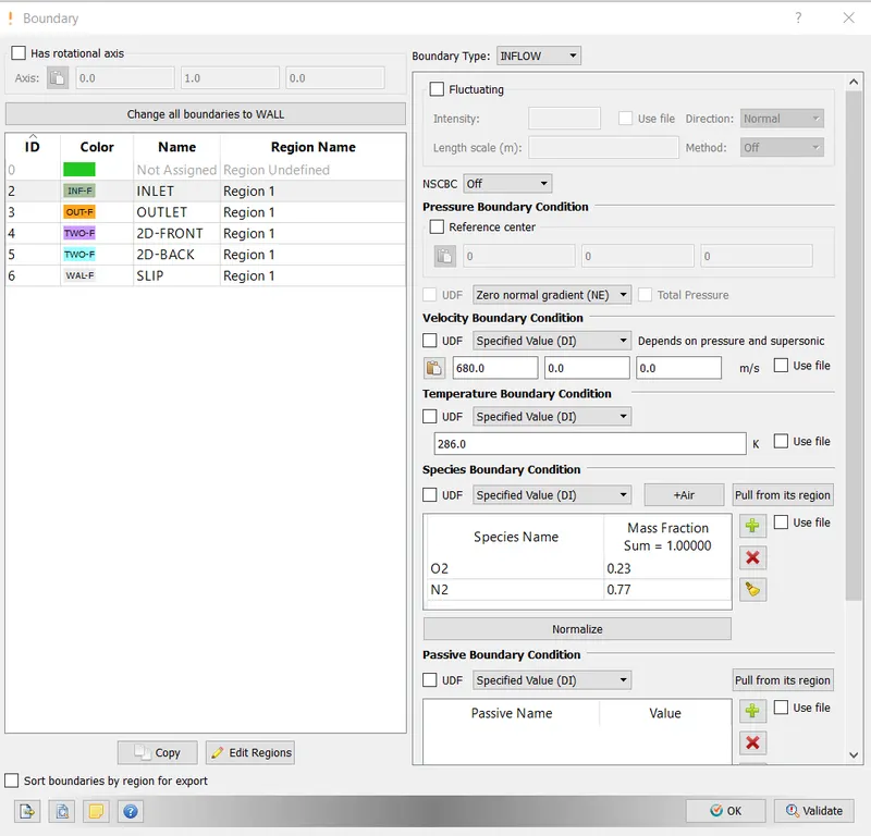
1. ) INLET : Boundary type is inflow. Pressure boundary condition is Zero normal gradient(NE) . Velocity Boundary conditions is Specified value(DI) . The velocity is the x direction is 680 m/s. The temperature boundary condition is also Specified value(DI). The temperature at inlet is 286 K. Species boundary condition is specified value(DI).The species is air (O2,N2).
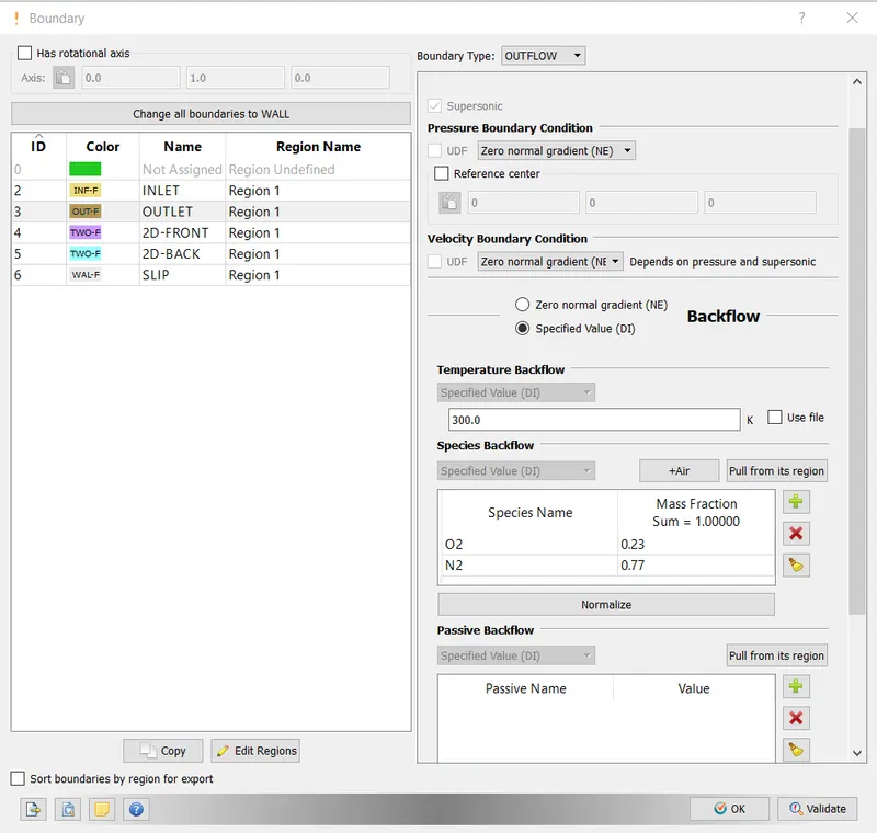
2. OUTLET : The boundary type is outflow. supersonic condition prevails at the outlet. The pressure boundary conditions and the velocity boundary conditions at the outlet is Zero normal gradient(NE). The backflow temperature is set to 300K and the condition is specified value(DI).
3. 2D-FRONT : 2D boundary conditions
4. 2D-Back : 2D boundary conditions
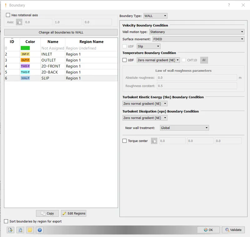
5. Slip : Boundary type is wall. Under the velocity boundary condition, the wall motion type is stationary and the surface movement is fixed. The tempearture bondary conditon is Zero normal gradiet(NE) . The turbulent kinetic energy bondary condituon and the turbulent dissipation boundary condition is Zero normal gradient(NE).

• Region initialization:

A region is created with the name region1. Velocity in x direction is 680 m/s and the temperature is 286 K. the species is air.

Every boundary is assigned to this region .

• Physical models:

Umder the physical models, only the turbulence modelling is required for this simulation.

Turbulence modelling:

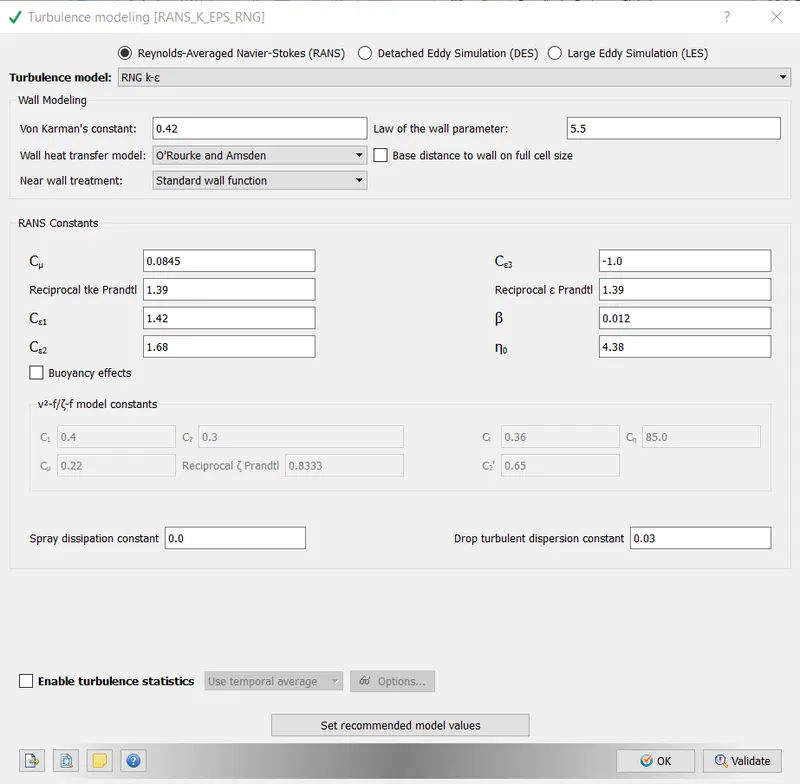
Reynolds average navier stokes (RANS) is selected.

Turbulence model : RNG K-epsilon

• Grid control:

Under the grid control, base grid is auto selected. Addition to that, adaptive mesh refinement is opted for.

The base grid size is : dx=0.8 meters;dy=0.8 meters;dz=0.8 meters.

Estimated cell count: 43647 without AMR

Adaptive mesh refinement:

In numerical analysis , adaptive mesh refinement (AMR) is a method of adapting the accuracy of a solution within certain sensitive or turbulent regions of simulation, dynamically and during the time the solution is being calculated.

In the adaptive mesh refinement, the maximum number of cells is limited to 200000. The region1 initialized , is tranferred from available regions to active region. Temperature is checked.

Embed type = Sub grid scale (SGS) and the time control tyoe is sequential. Maximum embedding level is 2.

Sub grid criterion is 0.05 K . the sub grid criterion is changed in the subsequent simulations from 0.05K to 0.03 K and 0.01 K.

• Output and post processing:

The post variables selection is kept by default what converge studio selects. The time interval for writing 3D output files is 100 cycles. File restart time is 1000 cycles.

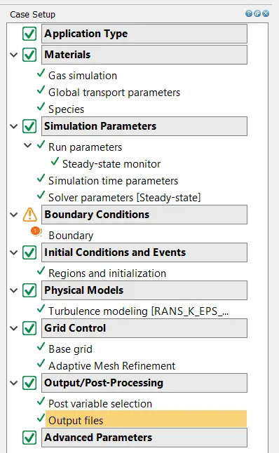
Following images are of the 1) case set up dock 2) Boundary condition at inlet 3) boundary condition at outlet 4) slip boundary copnditions

Simulation :

The input files are exported into a folder , The converge.exe and the mpiexe executables are pasted in the same folder containing the input files.

Command prompt is openned. By moving into the same folder that contains the input files, The command 'mpiexec.exe -n 4 converge.exe restricted' is ran.

For the base grid size 0.8 meters and the Sub grid criterion of 0.05 K , the simulation took 826.035 seconds to complete.

Post-processing:

Line plots are created in converge studio. The mass_avg_flow.out contains all the output files.

3D post processing:

Here a open source post processing software PARAVIEW is used . the output files are v=converted in paraview inline binary VTK format and stored within the out put sub folder.

Paraview is openned and in the output sub folder, the file with .vtm extension is openned. This is a group file containing all the converted output files .

• Surface with the edges:

This shows the meshed up surface at the initial time step:

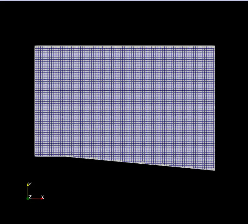
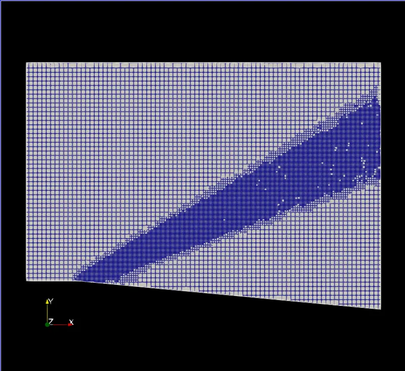
The first image shows the mesh generation. The second image is after the time steps. the shock and the expansion fan is quite visible.

The temperature is plotted as the variable , The subgrid criterion is 0.05K,0.03K and 0.01K respectively:

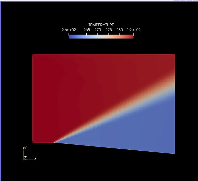
The above image shows the mach wave formation . In paraview this is done with surface option. the subsequent images have the mesh or the grids shown along with.

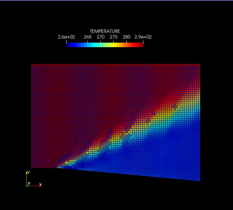
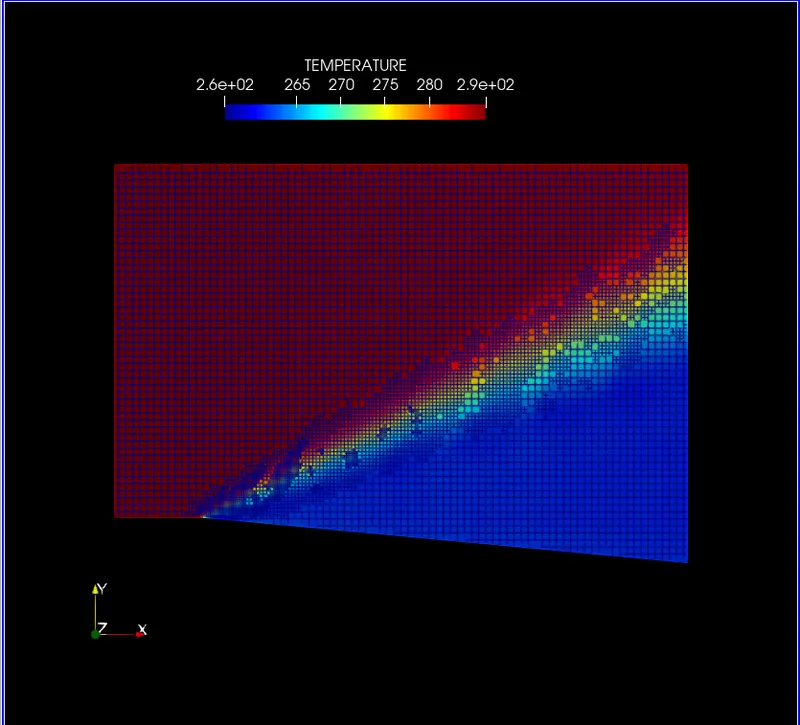
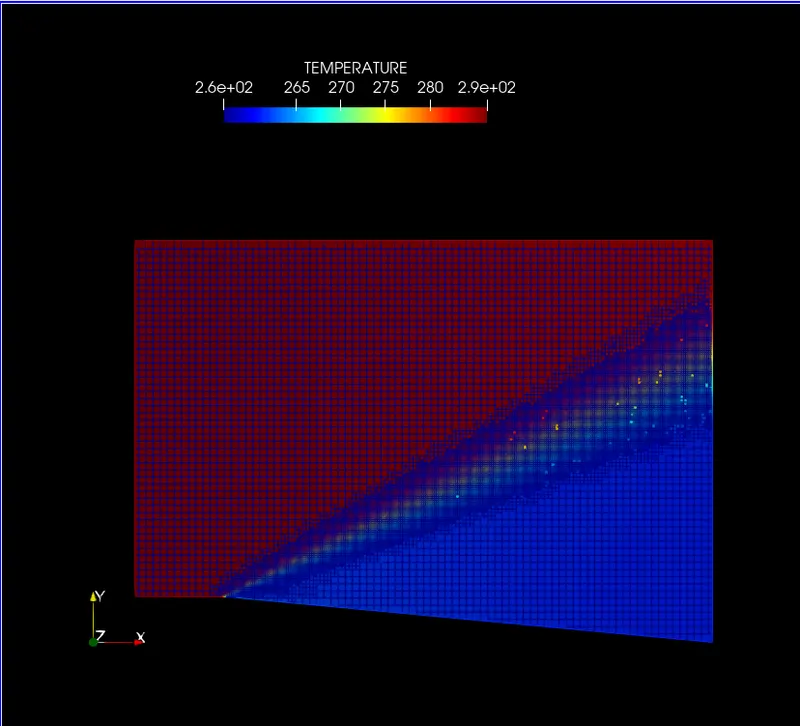
With lowering the subgrid criterion further the wave formation is more continuous and uniform.

An important observation can be made from the temperature contour, The inlet temperature is more than the outlet temperature. This is exactly as the phenomenon is expansion.

The pressure contours in the order of subgrid criterion 0.05K,0.03K,0.01K:

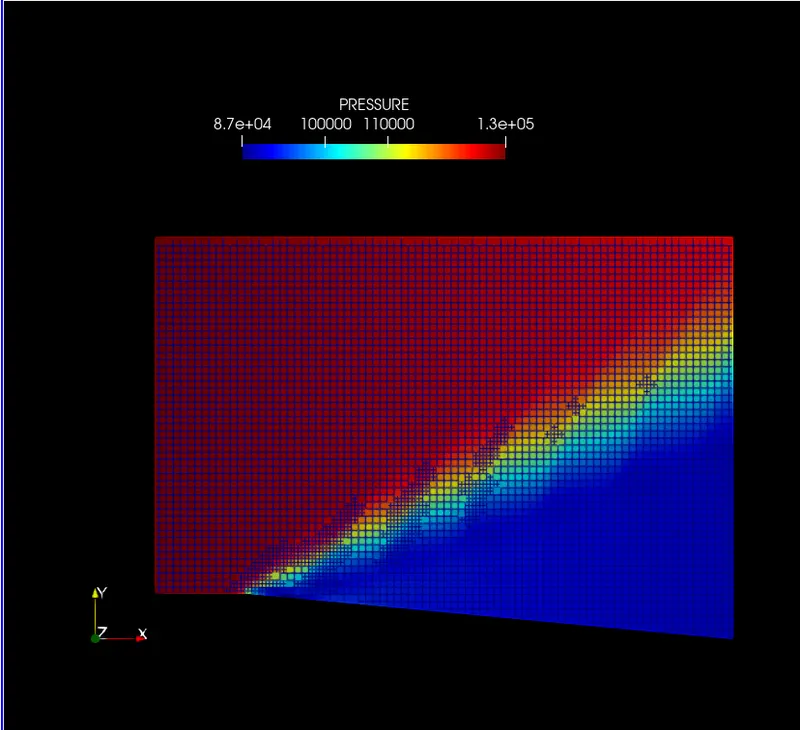
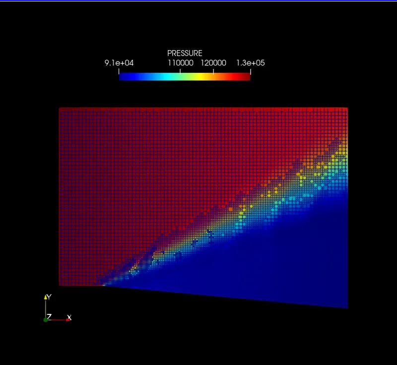
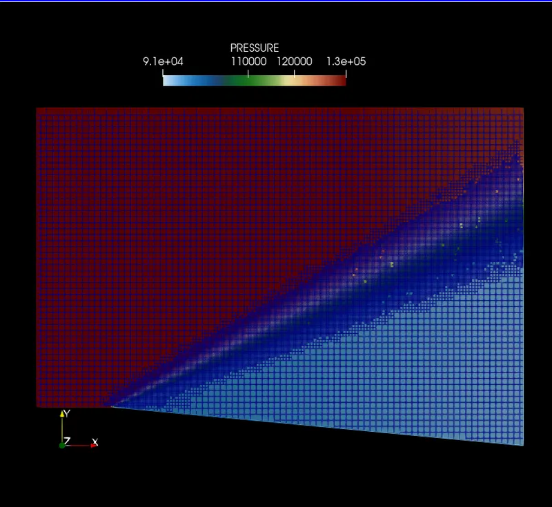
The pressure at the outlet also decreases after the prandtl-meyer shock wave formation.

Velocity contours in the order of subgrid criterion 0.05K,0.03K,0.01K

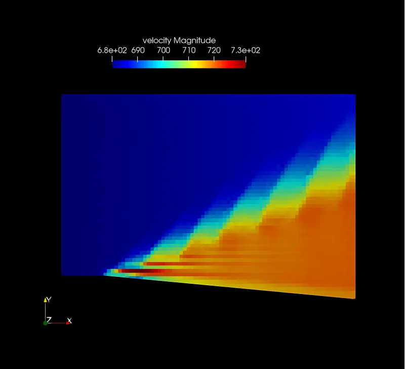
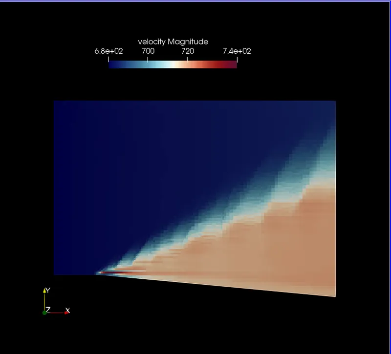
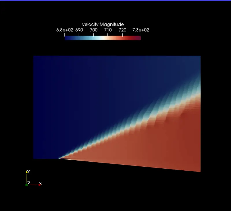
The velocity at the outlet increases. This attribute to the fact the mach number at the exit increases.

Line plots:

1) Mach number at inlet and exit . Order- sub grid criterion=0.05K,0.03K,0.01K:

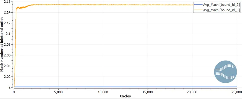
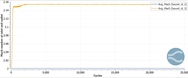
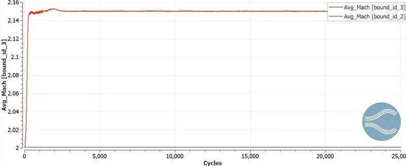
The Mach number at the outlet came oit to be 2.1563

2) Average temperature at inlet and outlet:

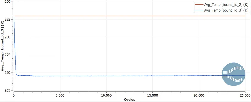
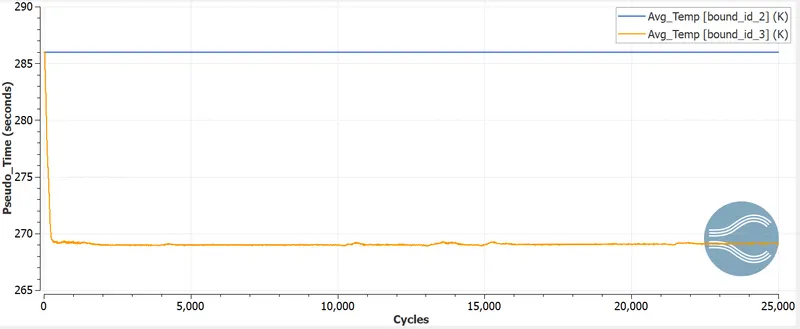
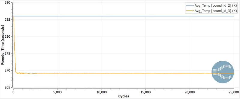
The exit temperature came out to be 269 K

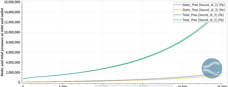
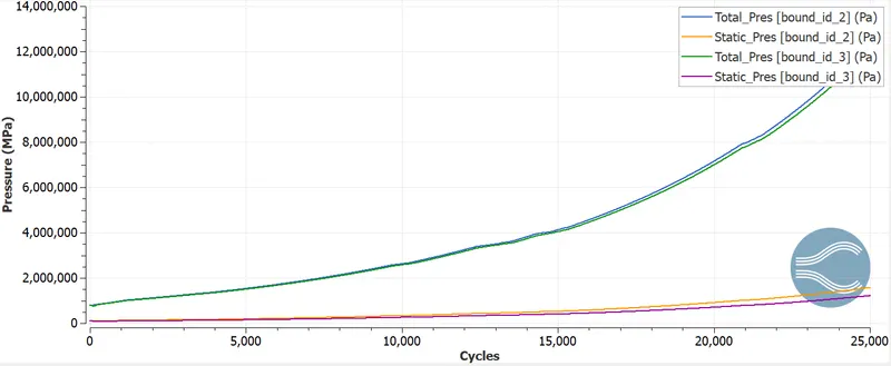
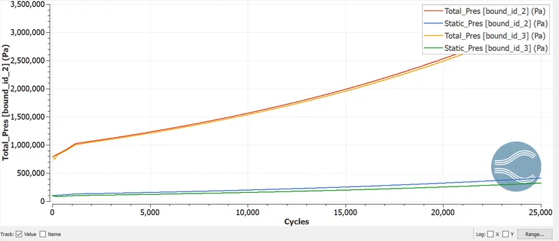
3) Average pressure at inlet and outlet:

In order of sub grid criterion =0.05K,0.03K,0.01K:

Effect of SGS on cell count:

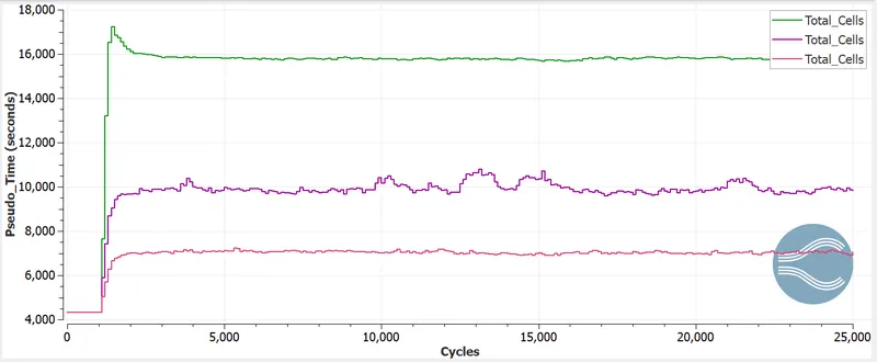
The green plot is for the subgrid criterion = 0.01K , the purple plot for sub grid criterion = 0.03K and the pink plot for the sub grid critreion = 0.05K.

With lowering the sub grid criterion, the number of cells or the cell count increases.

With lowering the sub grid criterion temperature, the shock wave region is more prominent .

The animation is uploaded in youtube . The link to that is :

https://youtu.be/wRdQZ-3Lll0

Analytical approach:

For this problem, The deflection angle is 5.46 degrees. Steps followed are

• Finding out the Mach number from the inlet velocity.

Mach number is defined as the ratio of the velocity of fluid flow to the velocity of sound at the same condition.

here , the velocity of flow is 680 m/s.

Velocity of sound at 286 K is 339.83m/s that is nearly 340m/s.

So, the Mach number is 2.

The ratio of specific heat gamma is 1.4

• From the Prandtl_meyer table , corresponding to the Mach number 2, the mach wave angle and the `nu(M1)` value is found out.

In this case the `nu(M1)`is 26.3798 degrees. and the mach wave angle is 30 degrees.

• using the prandtl meyer function to find out the values :

From the Prandtl meyer function:

`theta=nu(M1)-nu(M2)`

Here theta is the deflection angle. By solving the above equation, `nu(M2)`is 31.83 degrees.

From the prandtl meyer table, the mach number at the outlet can be calculated from the values at the `nu(M2)`=31.83 degrees.

`M2=2.18`

error = (2.18-2.16)/2.18*100 = 0.91%

The other properties can be calculated from the realtions that are cited at the begining.

Conclusion:

• Analysis is perforned with the assumption that the process is isentropic.
• With the increase in the number of cells, more accurate findings are obtained
• The temperature, pressure decreases through the expansio fan. The Mach number increases.