Week 5: Prandtl Meyer Shock problem

Aim:

To study about the shock wave, Shock flow boundary conditions, effect of SGS parameter on the shock location with help of simulation on the CONVERGE CFD.

Introduction:

As an object moves through a gas, the gas molecules are deflected around the object. If the speed of the object is much less than the speed of sound of the gas, the density of the gas remains constant and the flow of gas can be described by conserving momentum and energy. As the speed of the objects increases towards the speed of sound, we must consider compressibility effects on the gas. The density of the gas varies locally as the gas is compressed by the object. When an object moves faster than the speed of sound, and there is an abrupt decrease in the flow area, shock waves are generated. If the flow area increases, however, a different flow phenomenon is observed. If the increase is abrupt, we encounter a centered expansion fan.

There are some marked differences between shock waves and expansion fans.

What is a Shockwaves?

A shock wave is a type of propagating disturbance that moves faster than the local speed of sound in a medium, Like an ordinary wave, a shock wave carries energy and can propagate through a medium but is characterized by an abrupt, nearly discontinuous, change in pressure, temperature, and density of the medium. Across a shock wave, the Mach number decreases, the static pressure increases, and there is a loss of total pressure because the process is irreversible.

Through an expansion fan, the Mach number increases, the static pressure decreases and the total pressure remains constant. Expansion fans are isentropic, without heat addition and without friction.

Prandtl-Meyer Expansion Wave:

When supersonic flow encounters an abrupt change in direction but through a convex turn or a sudden expansion due to an abrupt reduction in pressure, expansion waves are produced. Expansion waves cannot reinforce one another to form a discrete expansion shock. First, as the flow expands, the trailing waves move into cooler air and their speed must be slower than the preceding expansion waves. Moreover, the formation of a discrete expansion wave would cause an increase in the total pressure, which is a violation of the second law of thermodynamics, and consequently is impossible. Instead of forming a discrete expansion wave, the flow expands incrementally through a series of weak expansion waves, which project out at the Mach angle, μ, relative to the local flow angle. When there is no turning of the flow and minimum wave angle represents the weakest possible oblique shock wave at a particular Mach number is called Mach Wave. Rather, a continuous expanding region called an expansion fan appears, composed of an infinite number of Mach waves called Prandtl–Meyer expansion waves. As the flow negotiates a convex corner or an abrupt change in pressure, these Mach waves fan out from the corner forming a fan starting with the Mach angle relative to the initial flow angle and ending with the corresponding Mach angle relative to the final flow angle. The Mach angle of the first expansion wave is easily determined as . Similarly, , where we must be careful to measure the angle relative to the new direction of flow downstream of the expansion. An example of this would be flow over a thin diamond-shaped airfoil. Prandtl–Meyer expansion fans could form as flow moves around the convex corners at the maximum thickness of the airfoil. These expansion fans could also form if the angle of attack of the flow was large enough to form a convex turn of the initial flow over the top of the airfoil. Similar expansion fans can form at the exit of an under-expanded nozzle or if an expansion is needed to equalize pressure or effect a change in the flow direction.

where 𝜈(Ma) is an angle called the Prandtl–Meyer function

Physically, (Ma) is the angle through which the flow must expand, starting with 𝜈 = 0 at Ma = 1, in order to reach a supersonic Mach number, Ma > 1.

Prandtl–Meyer reflections can occur at the exit of an under expanded (Under expanded nozzle: The exhaust pressure is still above ambient pressure). Initially, the flow must expand outwardly to match the back pressure at the exit. However, at the symmetry plane, it is impossible for the flow both above and below the plane to move away from the centreline. Consequently, the flow that moves out from the nozzle must expand again at the centerline to turn the flow parallel. A Prandtl–Meyer reflection can also occur in a flow in a duct when a convex corner turns the flow outward, causing the flow to need to expand again at the far wall to adjust the flow to move parallel to the far wall. In addition to reflections in an underexpanded nozzle, Prandtl–Meyer reflections can also occur downstream from an overexpanded nozzle (Overexpanded nozzle: The exhaust pressure is below ambient pressure) nozzle that originally adjusts to the exit pressure through an oblique shock, which turns it inwardly. The symmetry at the centerline causes the flow to turn parallel through a second oblique shock that drives the pressure above atmospheric. The flow then expands through a Prandtl–Meyer expansion to match the pressure, but turning outward. The flow then expands through a Prandtl–Meyer reflection to expand the flow back to a parallel direction to the nozzle flow direction

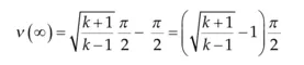
The maximum deflection angle can be estimated from the Prandtl–Meyer function. As the pressure ratio gets very high as it would at the edge of space, the resulting Mach number would get very high and the arctangent would return an angle close to 90°. Consequently, for flow, the maximum turning angle in radians becomes

In this section a flat plate airfoil and a thin diamond airfoil will be analysed using the shock expansion method which uses the analysis of oblique shocks and Prandtl–Meyer expansion fans to determine the pressure fields above and below the airfoil. supersonic airfoil showing oblique shock attached to leading edge below the airfoil and an expansion fan over the upper surface for the angle of attack. the angle of attack, α, is greater than the half wedge angle of the supersonic airfoil which means the flow over the upper surface of the airfoil encounters a convex turn causing a Prandtl–Meyer expansion fan, On the bottom of the airfoil the flow undergoes a concave angle producing an oblique shock wave.

Often over external flows where boundary layers are thin and attached, accurate pressure distributions and meaningful understanding can be achieved with inviscid or frictionless analyses. In short ducts with high speed and especially accelerating flows, this thin boundary layer assumption is often a reasonable and useful assumption. However, in many engineering situations when ducts are relatively long, friction can have an important impact in the analysis of flows. One area where this type of analysis is particularly important is compressible flow in pipelines. rise in static pressure can take place across a shock even though the total pressure diminishes. For a supersonic flow, friction will cause the velocity to decrease and the static temperature and pressure will rise in the constant area duct until a Mach number of 1 is reached, when the flow is subsonic friction will cause the static pressure to drop, increasing the velocity and dropping the static temperature until the flow reaches a Mach number of 1 where it is choked. In this section, a Fanno-line for adiabatic flow with friction in a constant area duct will be developed. Fanno-line in terms of temperature versus specific entropy describing the behaviour of both subsonic and supersonic flows. For both subsonic and supersonic flows, friction increases the entropy and the flow moves toward a Mach number of 1. Applications are Adiabatic flow with friction in a constant area duct, Flow with friction in converging nozzle with duct in series, Adiabatic flow with friction and area change. Fanno-line flow assumes that the flow is isentropic which also means that the flow will be adiabatic. This assumption is reasonable in many situations where the ambient temperature stays constant as the total temperature and the recovery temperature, which drives heat transfer, only varies by a few degrees in subsonic flows. In supersonic flows with friction L/D’s are typically small so an adiabatic flow is a reasonable assumption in these flows as well. The isothermal flow assumption suggests that the static temperature of a flow stays constant. This assumption is equally valid in long pipelines were the Mach number is low (M < 0.3) as in these low-speed flows the static temperature only varies a few degrees from the total temperature. Additionally, Fanno-line f low charts are relatively sparse in terms of at low Mach numbers and isothermal flow equations allow for simplified yet very accurate analysis at these low Mach numbers for situations where values can be large. using the isothermal flow assumption for flow in ducts or pipes where the peak Mach number is less than 0.1 should be considered.

Compressible flows are influenced by heat addition to a system as well as heat rejection from a system. Heat transfer can occur not only due to temperature differences between the wall of a channel and the flow but also due to thermal energy release caused by combustion. The process of condensation as well as evaporation can also influence compressible flows. The ideal gas law implies that the addition of thermal energy to a gas will cause an expansion. In a constant mass flow rate gas through a constant area duct, this addition of thermal energy will cause an increase in velocity. when heat addition occurs in this steady, frictionless, constant area flow. Heat addition will be shown to cause an increase in Mach number and a drop in static pressure while flow across a normal shockwave is known to cause a decrease in Mach number from supersonic flow to subsonic flow with a corresponding rise in pressure. Heat addition is somewhat similar to a converging duct in which both subsonic and supersonic flows will move toward sonic flow, M = 1, when thermal energy is added. The Rayleigh line relates changes in s – s* to changes in T/T*. This relationship can be developed from an intermediate equation in the development of a relationship for the changes of entropy for an ideal gas with a constant specific heat. The constant C is added to (s – s*)/R as s* is the maximum entropy for a given Rayleigh line and as a result (s – s*) will be negative. Note that for a given Rayleigh line both the mass flow rate and TT* will be the same for both the subsonic and sonic flow lines. One point is at the maximum for the T/T* line where T/T* is greater than one and d(T/T*)/d(s – s*) = 0. This just indicates that in this region the static temperature is more influenced by increasing Mach number than increasing TT*. The other point of tangency occurs where d(s – s*)/d(T/T*) = 0. This occurs at a Mach number of 1 as will be shown presently. Once a Rayleigh line reaches this second tangency any further increase in heating will result is a reduced flow rate. A subsonic flow cannot increase past this line to a supersonic flow and a supersonic flow cannot move past this location to a subsonic flow. However, it is possible for a normal shock to occur under certain conditions resulting in the supersonic flow becoming a subsonic flow but at a higher entropy level. This demonstrates that the maximum entropy occurs at a Mach number equal to one. A subsonic flow accelerating to a supersonic flow due to heat addition would violate the second law as would a supersonic flow decelerating to a subsonic flow due to heat addition. However, this does not preclude a supersonic flow from becoming a subsonic flow through a normal shock. Applications are Frictionless flow with heat addition and area change , constant area flow with heat addition and friction.

Case Setup:

1.Open the Converge Studio and then import the file by using option, file->Import->Import STL. Navigated the file and files imported always in the form of metres

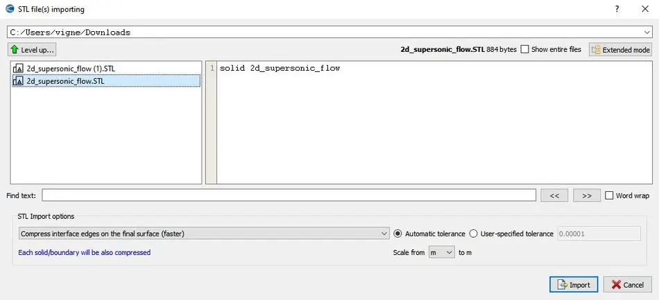
visible items are selected then check the geometry bounding box

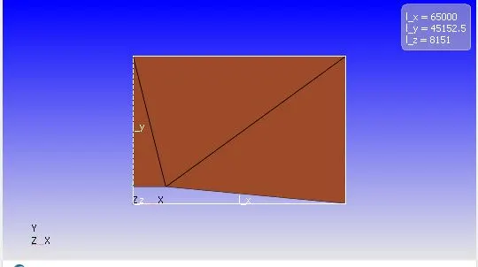
2.On the above figure, Geometry Bounding Box measurements would be displayed on the Top-Right Corner. It shows the values in the order of 1000. So it is showing the measurements may be in the form of mm. Scaled the entire geometry by using the option Geometry->Transform->Scale. Then select the input method as entire surface. Provide the uniform scale factor as 0.001 (It is the conversion ratio from millimetre to meter) and then click apply.

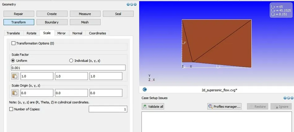
3. View toolbar->Normal Toggle is selected then it will display the direction of the normal in the geometry.

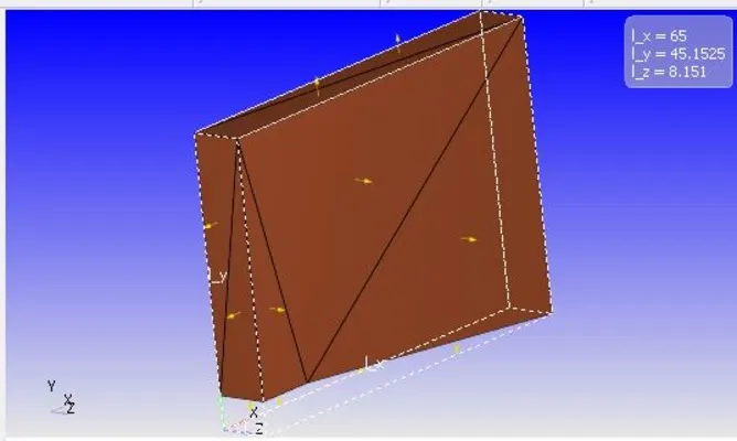
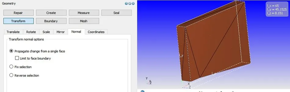
4.Geometry->Transform->normal is selected then select propagate change from single face and select the surface then click apply.

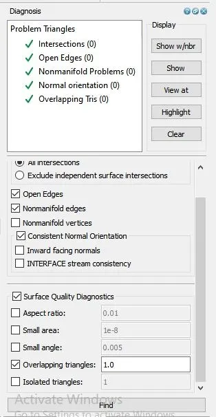
5.Click on the Diagnosis dock and then click find.

To view the errors, present in the geometry

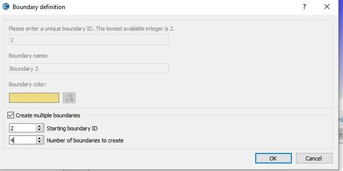
6.Geometry->Boundary->Flag is selected then click on create a new boundary. The boundary definition dialog box appears then select create multiple boundaries and entered as 4 (as per needed boundaries) and then click ok.

7. Now renamed the boundary flag as per geometry by simply right clicking the created flags and selected the surfaces and appropriate flags and clicked apply for each and every flag.

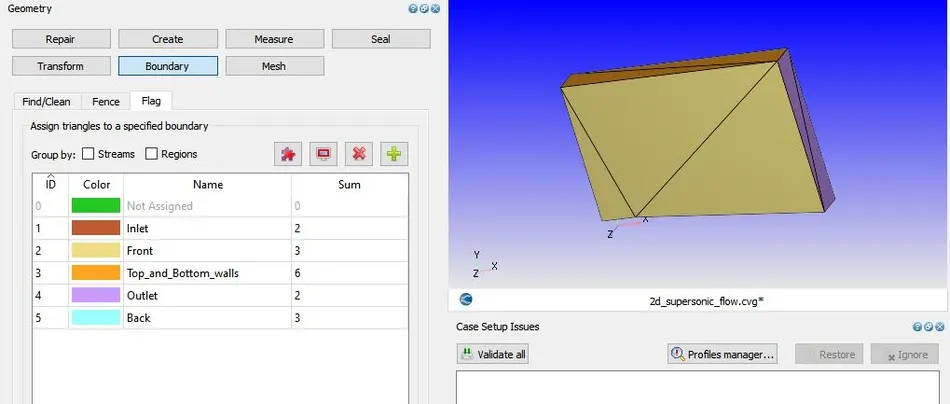
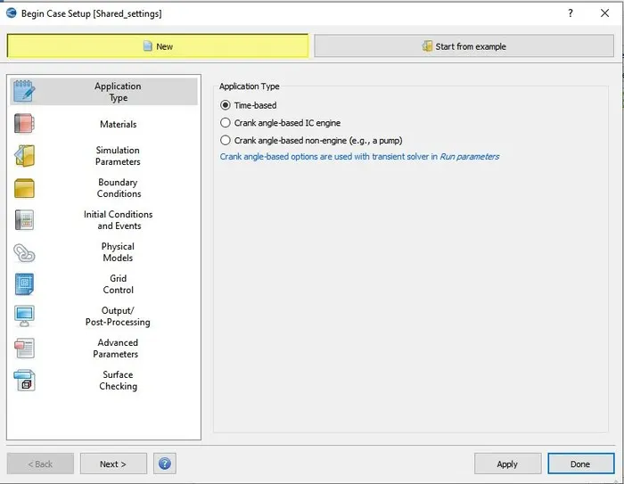
8.On the Case setup tab is selected. Begin case setup dialog box appeared

9.Select the Application type as time-Based. (It provides the option for steady/Transient simulation for the general flow).

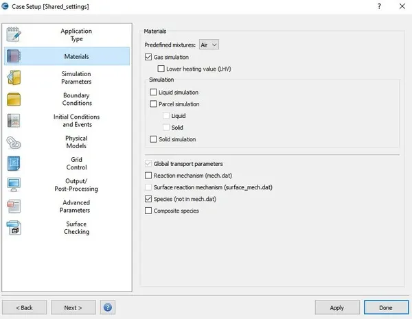
10. Under the materials, selected air as a pre-defined mixtures and then species is selected.

Working fluid is air with the species of oxygen and nitrogen

Species is the separate file which will required each and every time by the solver.

11. Loaded Predefined mixture dialog box appears on that one click yes. (This step will overwrite some the files).

12.Gas simulation is selected, Redlich-Kwong is selected as an equation. It performs well high temperatures for both ideal and Non-ideal Gases.

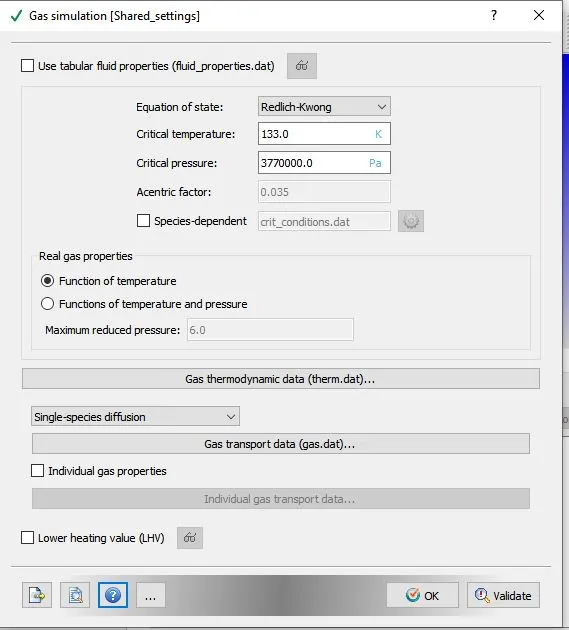
13.Global transports parameters are selected, turbulent Prandtl number as 0.9, turbulent Schmidt number as 0.78. click ok.

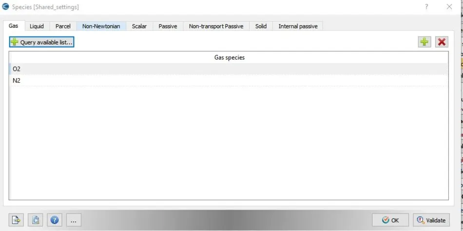
14. Species is selected then species dialog box opens there selected the add symbol, species is added then click ok.

15.Run parameters is selected and solver is selected as steady state, simulation mode as Full hydrodynamic and solving the energy and momentum equations.

Running the simulation in steady state and involving the solver by selecting the simulation mode as full hydrodynamic

16.Simuation time parameters is selected then dialog box appears then enter the number of cycles as 25000, Timestep has been provided.

17.Solver Parameters is selected then dialog box appeared then selected a solver such as PISO algorithm and density-based solver

PISO Algorithm with more than one corrector step to converge quickly and density-based solver is used because of simulating the supersonic flow.

18.region and initialization is selected then dialog box appears then renamed the region and then vales entered for velocity, pressure, temperature e.t.c..,

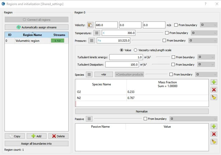
The Computational domain will be initialized with these values.

19.Physical models is selected then unchecked the turbulence modelling.

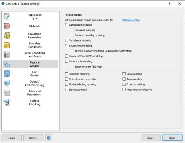
20.Boundary is selected then boundary dialog box appears then volumetric region is assigned to each and every boundary.

Shock flow boundary conditions:

Boundary conditions are constraints necessary for the solution of a boundary value problem. A Boundary value problem is a set of differential equations to solved with help of describing the boundary conditions. There are five types of boundary conditions (i) Dirichlet Boundary Condition, (ii) Neumann Boundary Conditions (iii) Robin Boundary condition, (iv) mixed boundary condition, (v) Cauchy boundary condition.

Dirichlet Boundary Condition-This condition specifies the value that the unknown function needs to take on along the boundary of the domain.

Neumann boundary conditions- It specifies the values that the derivative of a solution is going to take on the boundary of the domain.

Robin Boundary Conditions-It consists of a linear combination of the values of the field and its derivatives on the boundary.

Mixed Boundary conditions-the mixed condition implies different types of B.C. applied to different parts of the boundary.

Cauchy Boundary condition-Cauchy condition implies the imposition of two constraints (1 Dirichlet B.C. + 1 Neumann B.C.).

on the most of the papers for shock flow analysis, Dirichlet Boundary condition given as input and Neumann Boundary conditions is given at the outlet. Some paper describes that Outlet boundary conditions should to insensitive. It may be also one of the reason for utilizing the Neumann Boundary conditions at outlet. It looks like Cauchy Boundary Condition.

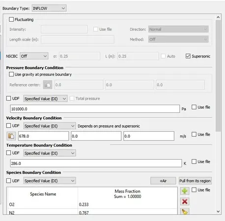
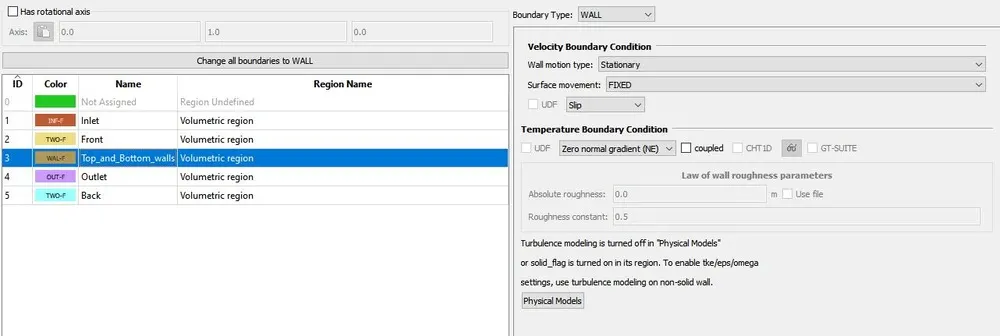
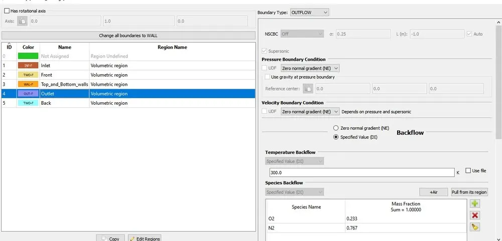
Front and back boundary flaging is assumed as 2D Boundary condition

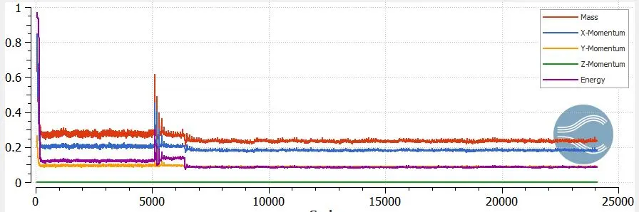
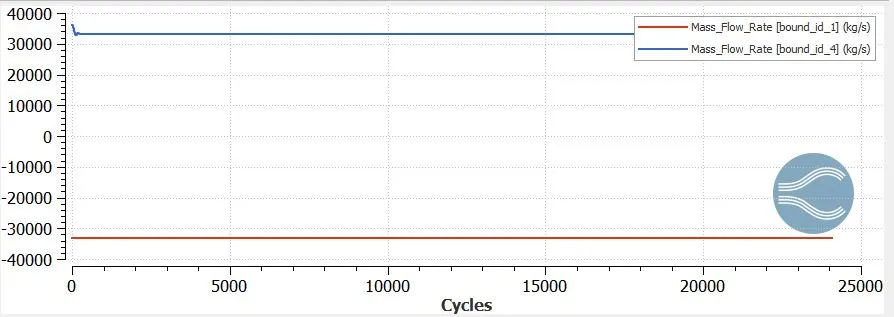
21.Steady state monitor is selected then add config and added the monitor variables such as flow variables.

22.Grid control is selected from the case setup and checked the adaptive mesh refinement.

23.Base grid is selected then entered the values of size such as 0.8 m uniformly

24.Adaptive mesh refinement is selected then dialog box appears then dialog box appears entered the maximum cells, region is set as active region, Select the parameters, entered the criteria and embedding level and click ok.

25.Post-variable selection is selected then dialog box appears, selected the output variables and then click ok.

26.File->export->export input files is selected then dialog box appears then navigate the folder and then click ok.

26.copy the converge.exe and mpiexec.exe application files is copied from the installation files to the case setup

27.open the cygwin terminal and navigate it to the case setup and run the command called mpiexec -n 2 converge --license explore

Plots:

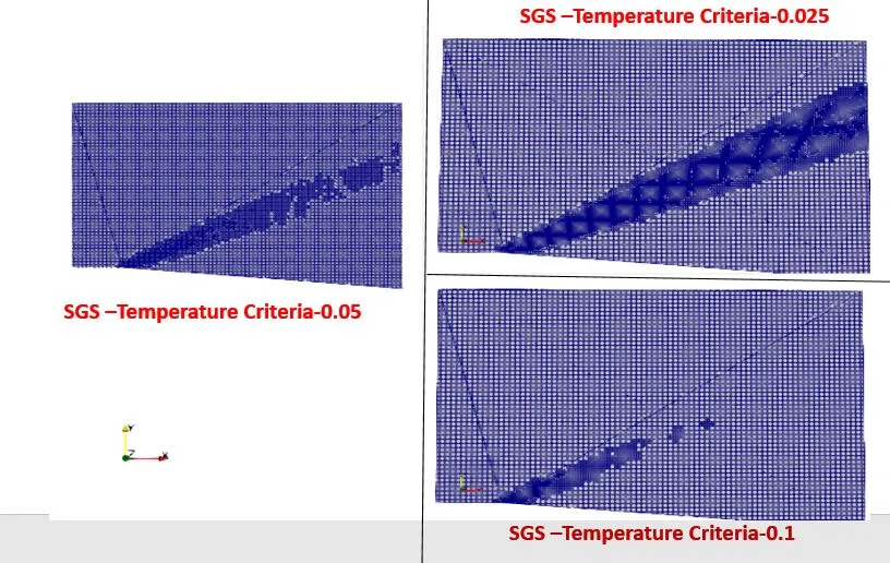
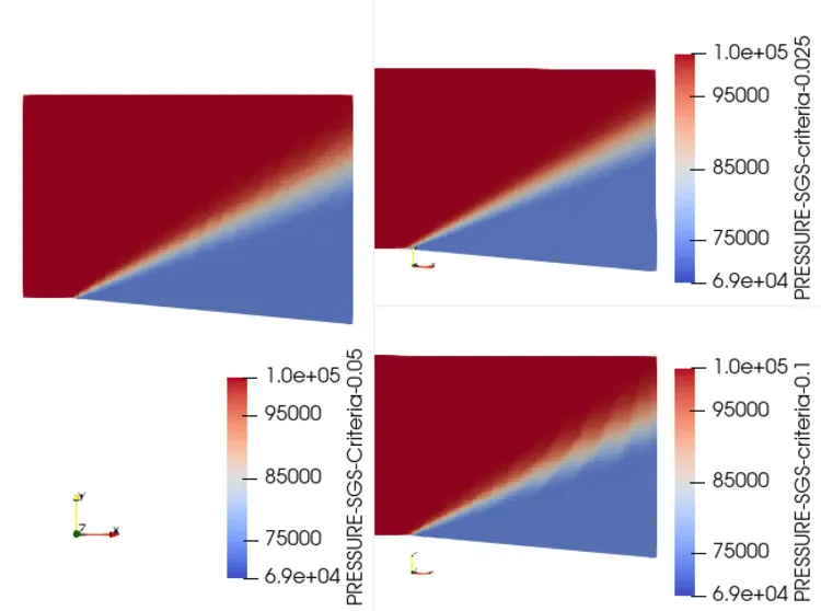
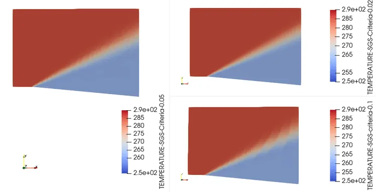
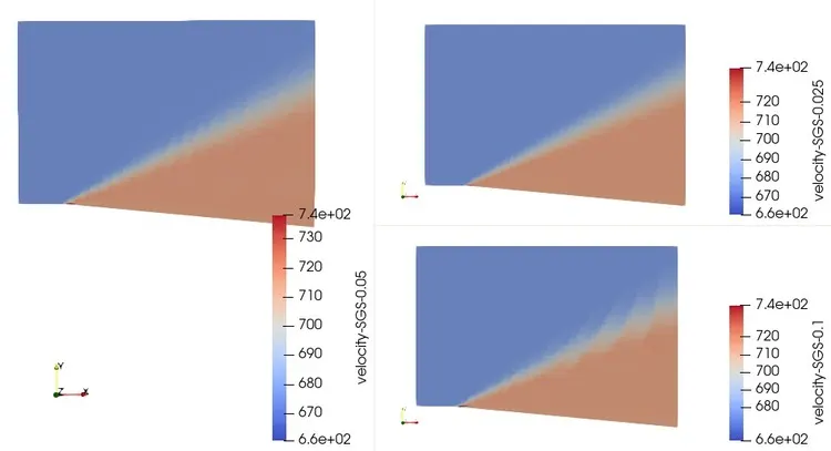
(i)Velocity-678 m/s, Temperature gradient Sub Grid Scale criteria -0.025

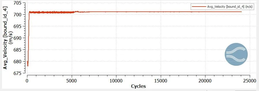
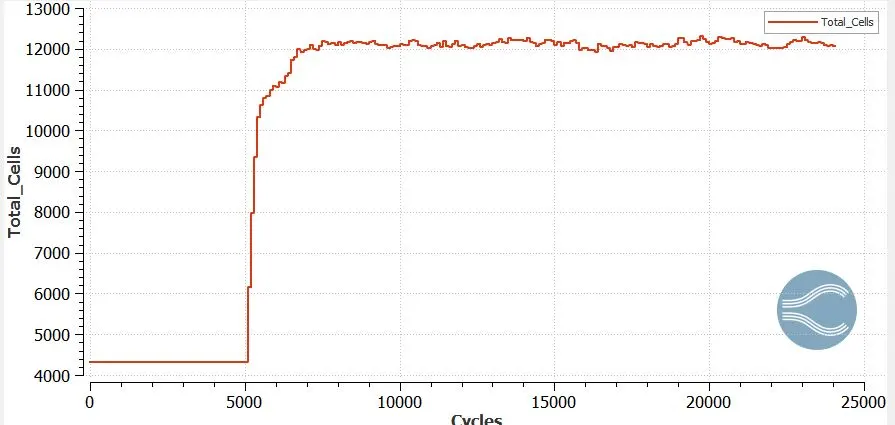
(ii)Velocity-678 m/s, Temperature gradient Sub Grid Scale criteria -0.1

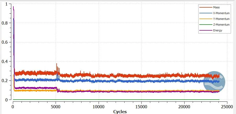
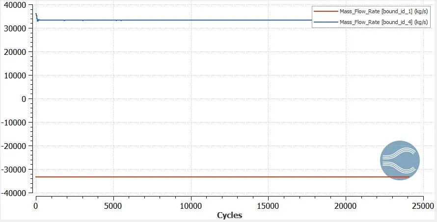
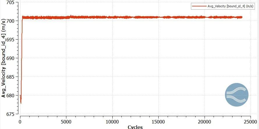
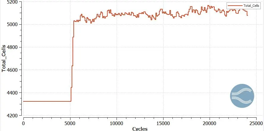
(iii)Velocity-678 m/s, Temperature gradient Sub Grid Scale criteria -0.05.

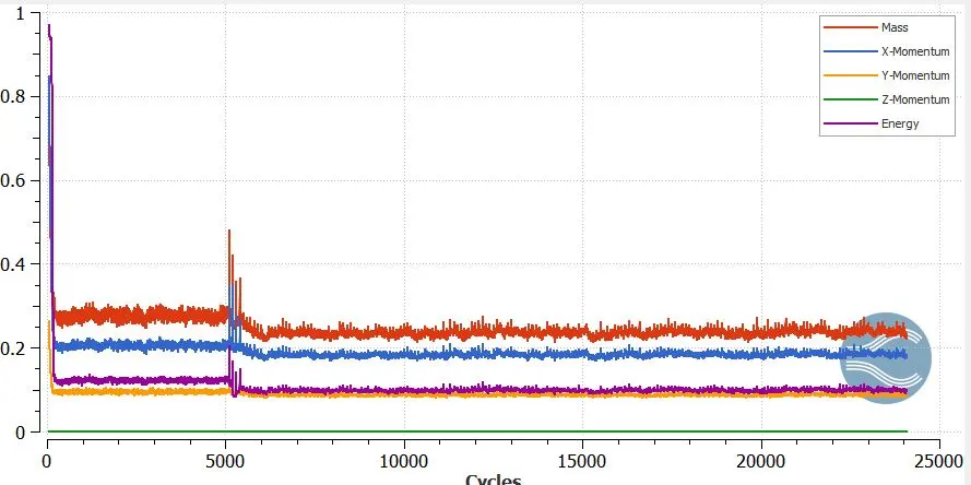
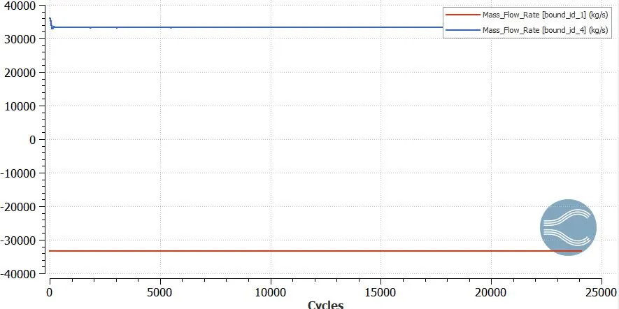
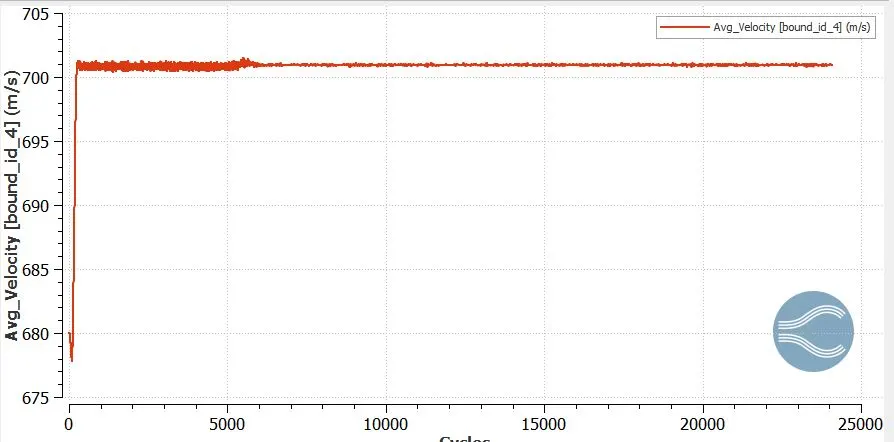
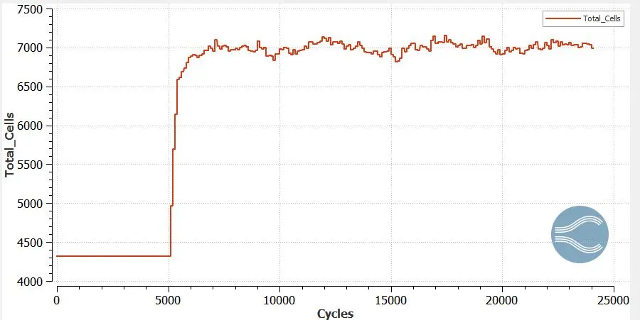
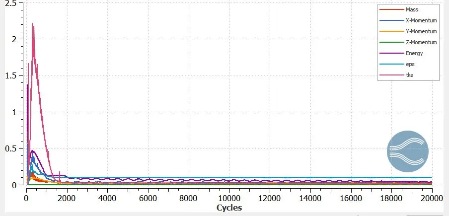
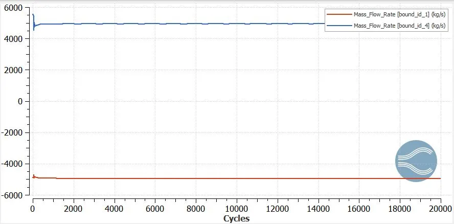
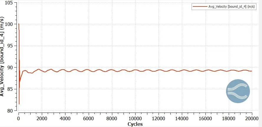
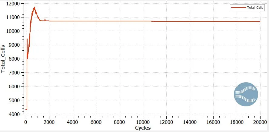
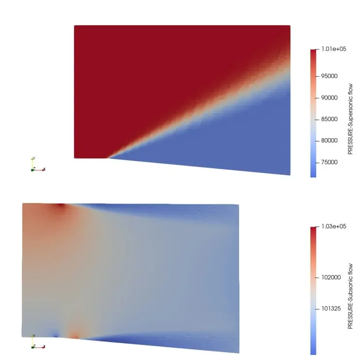
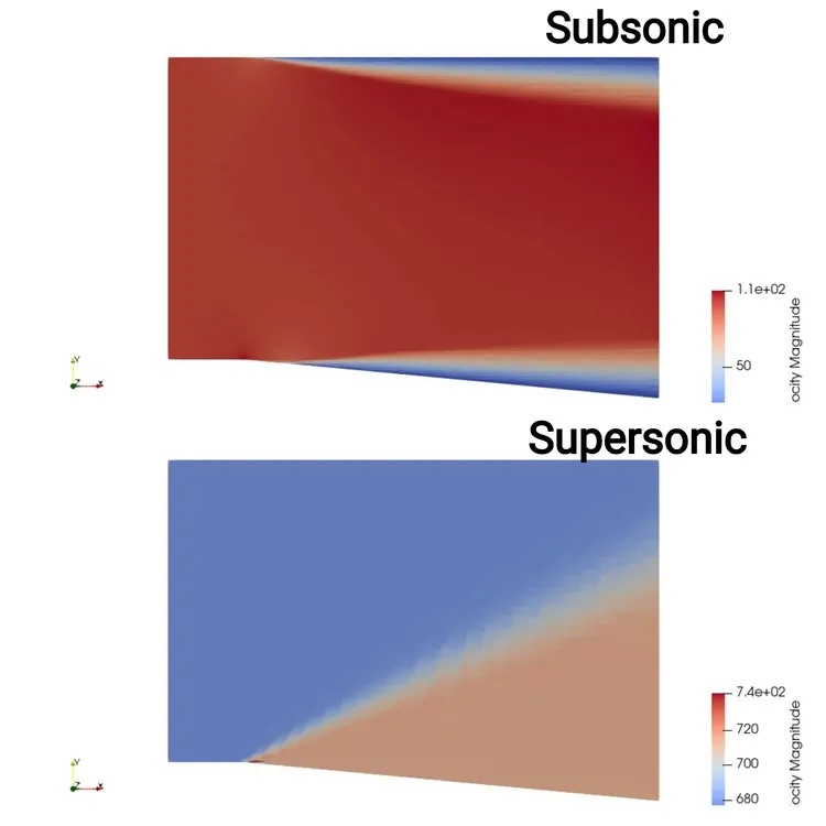
(iv)Velocity-100 m/s, Temperature gradient Sub Grid Scale criteria -0.05, Viscosity model- RNG

Contours:

Conclusion:

(i)SGS criteria such as temperature gradient decreases will creates the much mesh refinement with increase in cell count.

(ii)Due to refining with the help of SGS criteria, it is able to capture the expansion wave clearly.As the SGS criteria decreases by reducing the disturbances in the expansion wave.

(iii)It is clearly shows that the pressure, Temperature drop due to the expansion wave but velocity increases. In a similar way Mach number also increases.

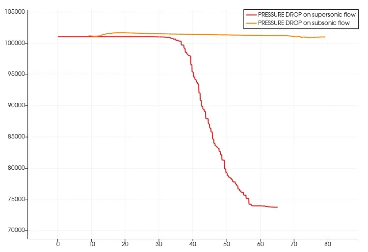
(iv)Due to subsonic flow, Pressure drop is very small compared to the supersonic flow.

(v)In subsonic flow, can observe that due to the shape, the boundary layer starts at two different points parallel to the axis.

(vi)In Subsonic flow the velocity increases with decrease in pressure.

(vii) in the pressure drop of subsonic flow, change in shape reduces the pressure drop which is the small curved line

I have attached the link for the Adaptive Mesh Refinement videos

Criteria-0.1-https://youtu.be/PMF-Y1It_0E

Criteria-0.05-https://youtu.be/FEaaF1O4frs

Criteria-0.025-https://youtu.be/e11Wnwr-7S4