Week 5: Prandtl Meyer Shock problem

AIM:

            To simulate the Prandtl Meyer Shock flow in converge CFD.

OBJECTIVE:

• To simulate the supersonic and subsonic flow through a duct.
• To observe the effect of SGS on shock location.
• To study the formation of shock waves in the duct.

THEORY:

SHOCK WAVE:

shock is a type of propagating disturbance that moves faster than the local speed of sound in the medium. A shock wave carries energy and can propagate through a medium but is characterized by an abrupt, nearly discontinuous, change in pressure, temperature and density of the medium. Shock wave strong pressure wave in any elastic medium such as air, water, or a solid substance, produced by supersonic aircraft, explosions, lightning, or other phenomena that create violent changes in pressure. shock waves travel faster than sound, and their speed increases as the amplitude is raised; but the intensity of a shock wave also decreases faster than does that of a sound wave, because some of the energy of the shock wave is expended to heat the medium in which it travels.

PRANDTL MEYER EXPANSION FAN:

A supersonic expansion fan, technically known as Prandtl–Meyer expansion fan, a two-dimensional simple wave, is a centred expansion process that occurs when a supersonic flow turns around a convex corner. The fan consists of an infinite number of Mach waves, diverging from a sharp corner. When a flow turns around a smooth and circular corner, these waves can be extended backwards to meet at a point. Each wave in the expansion fan turns the flow gradually (in small steps). It is physically impossible for the flow to turn through a single "shock" wave because this would violate the second law of thermodynamics.

 

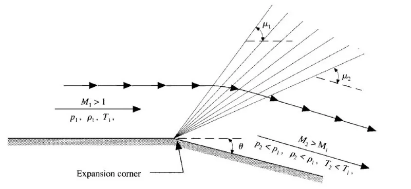
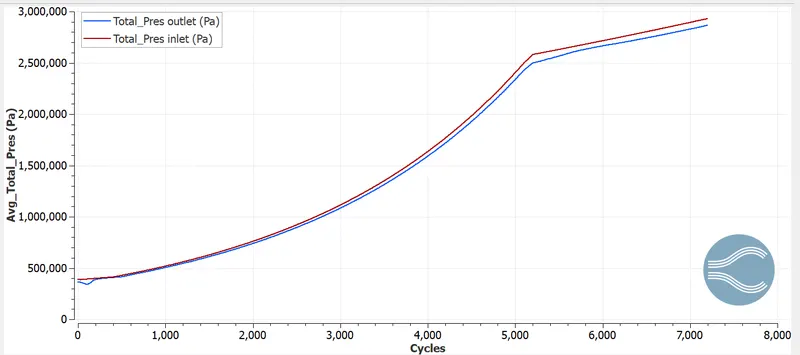
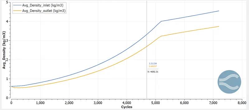
Across the expansion fan, the flow accelerates (velocity increases) and the Mach number increases, while the static pressure, temperature and density decrease. Since the process is isentropic, the stagnation properties (e.g. the total pressure and total temperature) remain constant across the fan.

SHOCK FLOW BOUNDARY CONDITIONS:

BOUNDARY CONDITIONS:

• A boundary value problem is a differential equation together with a set of additional constraints called the boundary conditions.
• A solution to a boundary value problem is a solution to the differential equation which also satisifies the boundary conditions.
• A boundary value problem has conditions specified at the extremes of the independent variable in the equation.

TYPES OF BOUNDARY CONDITION:

           DIRICHLET BOUNDARY CONDITION:  

                  In this type, When imposed on an ordinary or a partial differential equation, it specifies the values that a solution needs to take on along the boundary of the domain.

           NEUMANN BOUNDARY CONDITION:

                  In this type, when imposed on an ordinary or partial differential equation, the condition specifies the values in which the derivative of a solution is applied within the boundary of the domain.

           ROBIN BOUNDARY CONDITION:

                  In this type, when imposed on an ordinary or a partial differential equation, it is a specification of a linear combination of the values of a function and the values of its derivatives on the boundary of the domain.

           MIXED BOUNDARY CONDITION:

                  In this type, a boundary value problem in which the solution of the given equation is required to satisify different boundary conditions on disjoint parts of the boundary of the domain where the condition is stated.

           CAUCHY BOUNDARY CONDITION:

                  In this type, a Cauchy boundary condition augments an ode or a pde with conditions that the solution must satisify on the boundary so that a unique solution exists. A Cauchy boundary condition specifies both the function and the normal derivative on the boundary of the domain.

WHY NEUMANN BOUNDARY CONDITION IS USED FOR SUPERSONIC OUTLET?

Neumann b.c. is used because the values of all the variables like pressure, velocity, temperature and mach no are not available before solving the problem. So nothing is specified at a supersonic outlet and all variables are extrapolated from the domain interior. Only the normal derivative of variables are specified as zero gradient.

If any pressure or velocity is specified at outlet the solution will not converge and become unstable.

GEOMETRY SETUP:

• IMPORT GEOMETRY:

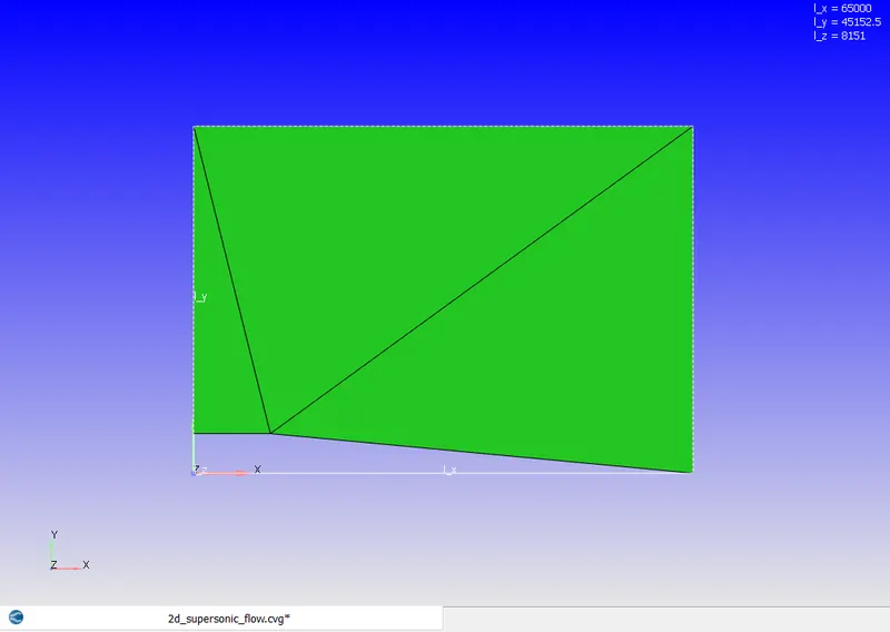
        Geometry is imported to the workspace from the stl file given.

                     

• SCALING THE GEOMETRY:

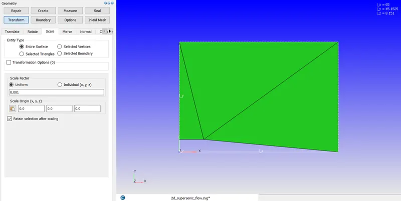
        Converge uses dimensions in meters the scale is too large. So, need to scale down.

        The geometry is scaled down by going to transform > scale and apply a scaling factor.

        

• CREATING BOUNDARIES:

        The boundary are created for the geometry under boundary flag tab.

           

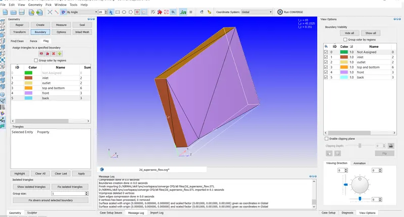
         The boundaries are assigned to the faces and the name of the boundaries are edited and click apply.

• NORMAL ORIENTATION:

        The orientation of normal are checked and its changed such that the normal points inwards by going to transform > normal

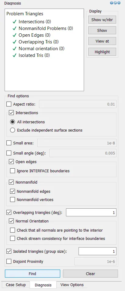
• DIAGNOSIS:

        The diagnosis is runed and checked for problems for the geometry.

         

BEGIN CASE SETUP:

• APPLICATION TYPE:

        On the right panel go to the case setup tab, select begin case setup.

         

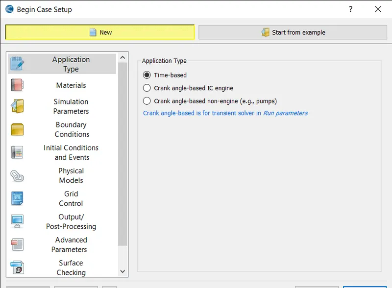
         Select the application type as time-based and select apply and done.

• MATERIALS:

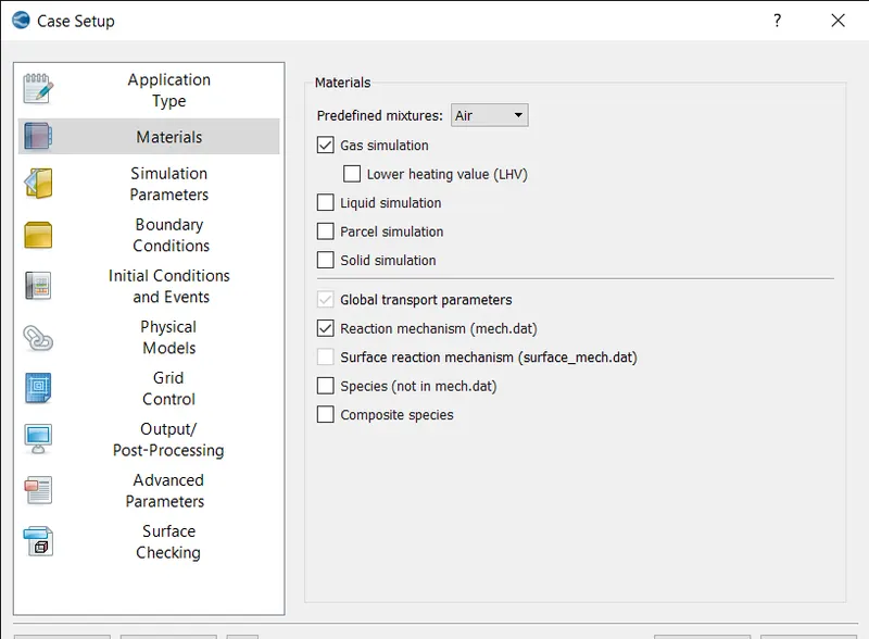
        Select materials and select the checkbox reaction mechanism then select the predefined mixture as air then click apply and done.

        

• GAS SIMULATION:

         

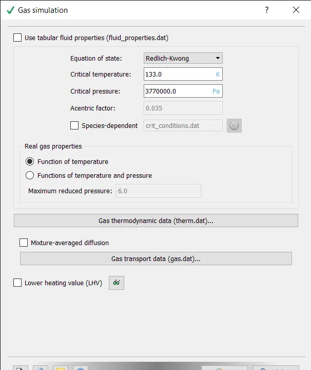
         The default values are selected and press ok.

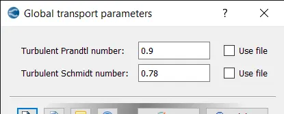
• GLOBAL TRANSPORT PROPERTIES:

        Select global transport properties, keep the default values and press ok.

         

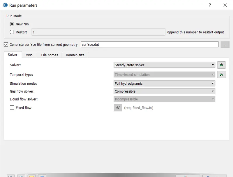
• RUN PARAMETERS:

        Under solver tab select solver as steady-state solver

        

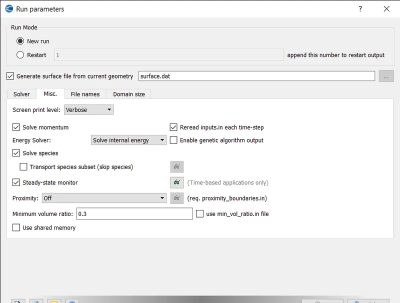
• MISC TAB:

        Under misc tab checking the steady-state monitor option and disabling use shared memory option and click ok.

        

• SIMULATION TIME PARAMETERS:

        

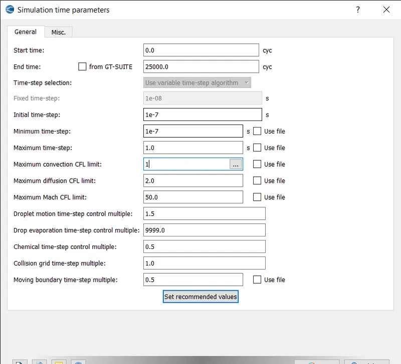
        Set the start time, end time, initial, minimum and maximum time steps as shown above.

• SOLVER PARAMETERS:

         

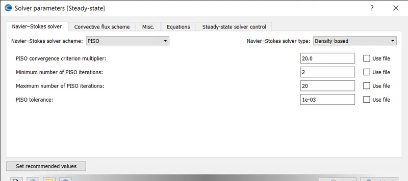
         Select the Navier-stokes solver type as density based and click ok.

• SOLVER PARAMETERS MISC:

        

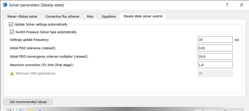
        under misc tab maximum CFL limit set to 1.

• REGIONS AND INITIALIZATIONS:

         

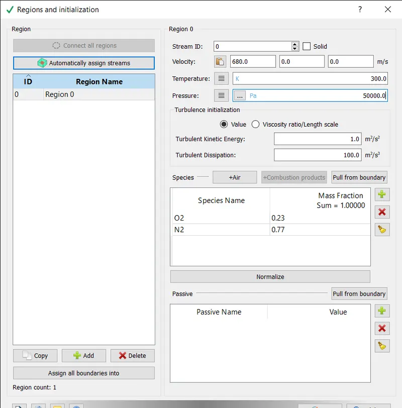
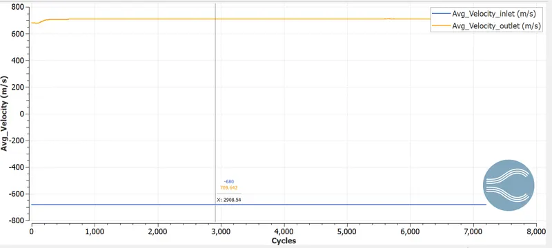
          The inlet velocity of 680m/s is specified in velocity tab along x- direction.

         The regions are created and air is added as species and mass fractions are changed to O2 as 0.23 and N2 as 0.77.

• BOUNDARY CONDITIONS:
• INLET:

         

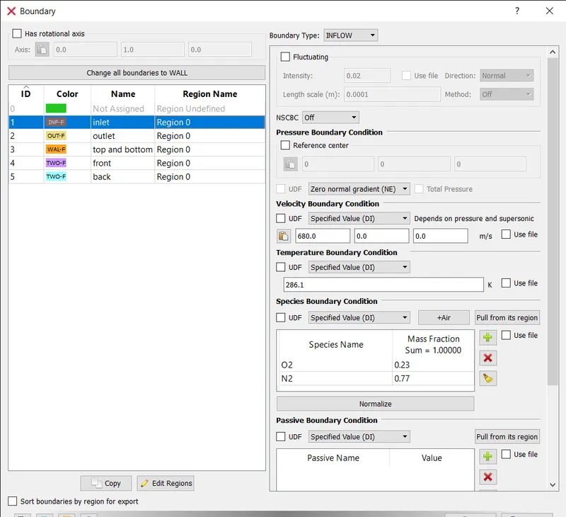
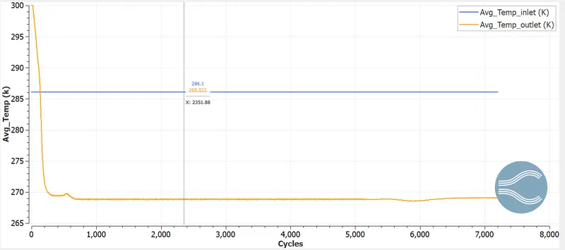
         For inlet, set the pressure boundary condition as zero normal gradient, velocity as 680m/s, temperature as specified value of 286.1k and select air for species boundary conditions.

         OUTLET:

          

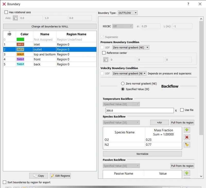
          Set the outlet pressure boundary conditions as zero normal gradient, velocity as zero normal gradient and for species backflow select air.

         TOP AND BOTTOM:

          

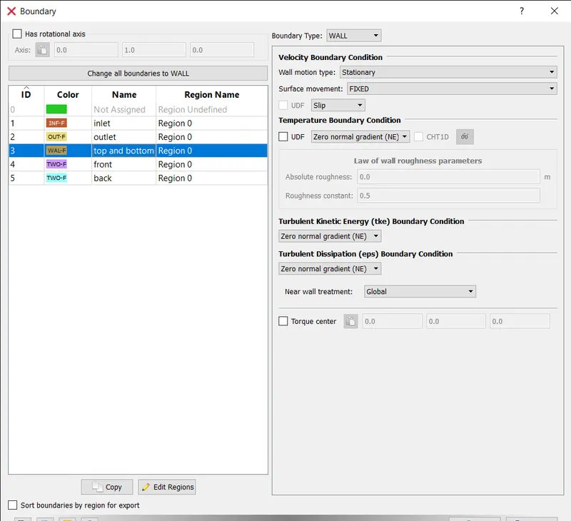
          Select the boundary type as wall type with slip velocity boundary conditions. And the temperature as zero normal gradient.

          FRONT AND BACK:

                  

            

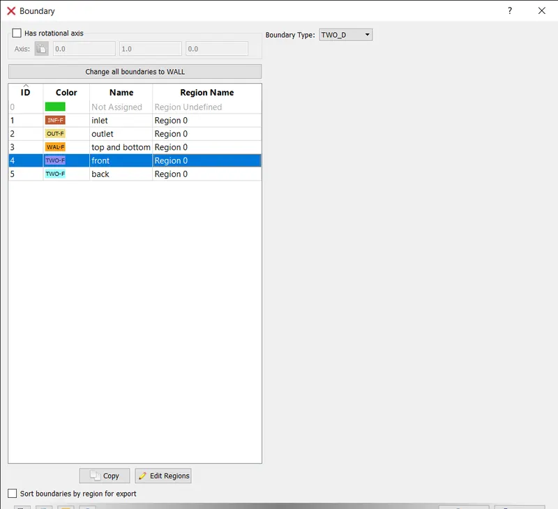
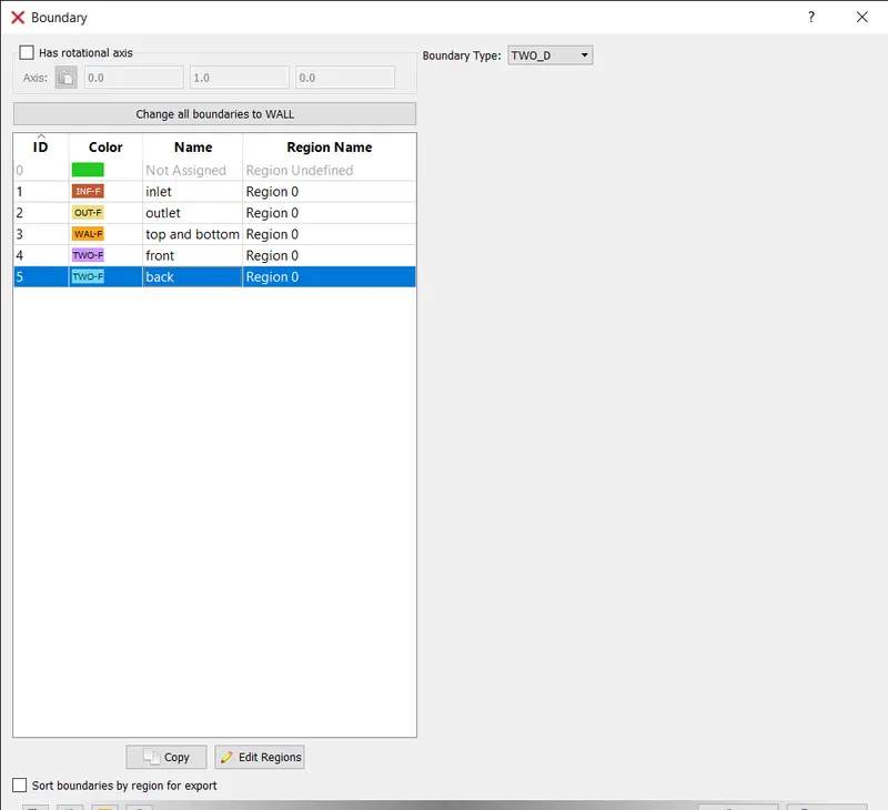
          The boundary type is defined as two_d.

• STEADY STATE MONITOR:

         

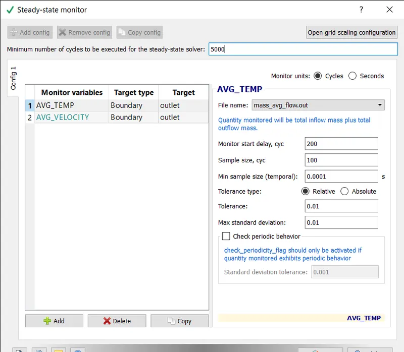
          The monitor variables are added and the minimum number of cycles, monitor start delay and sample sizes are defined.

• PHYSICAL MODEL:

        

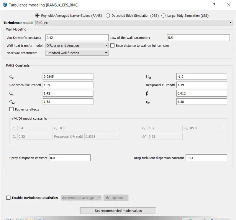
        The RNG K-epsilon and default values are fixed and click ok.

• GRID CONTROL:

         

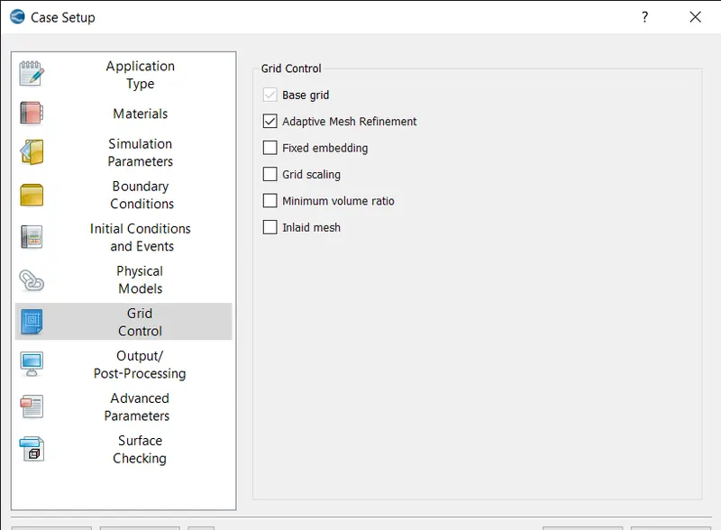
        Adaptive mesh refinement is checked in the grid control tab.

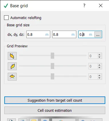
• BASE GRID:

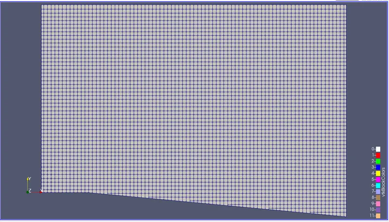
         The base grids are defined as 0.8 meters and press ok.

          

• ADAPTIVE MESH REFINEMENT:

        

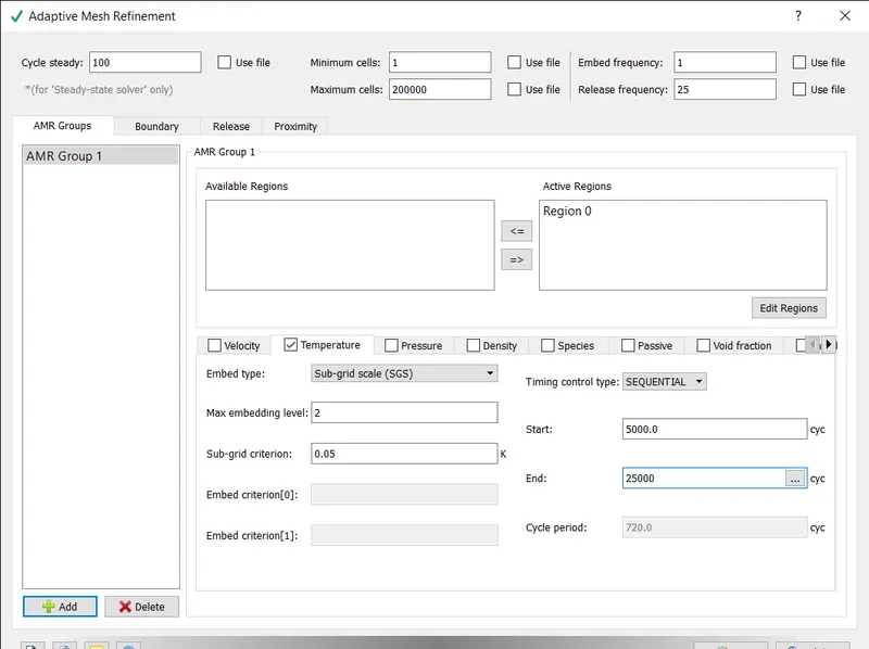
        Minimum cells set to 1 and maximum cells as 200000. temperature scheme is used for AMR and embeded type as SCS  and maximum embedding level to 2 and sub-grid criterion is varied for each case.

• POST VARIABLE SELECTION:

         

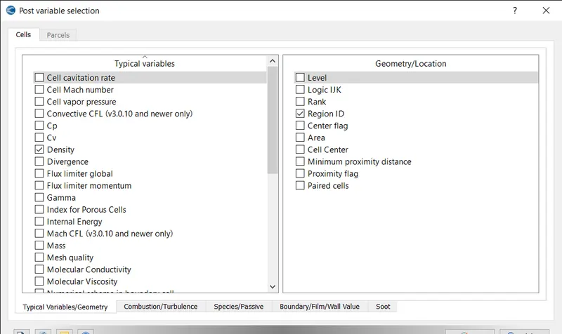
         Keep the default values in typical variables tab.

          

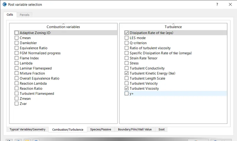
          In combustion or turbulence tab default values are kept and click ok.

• OUTPUT FILES:

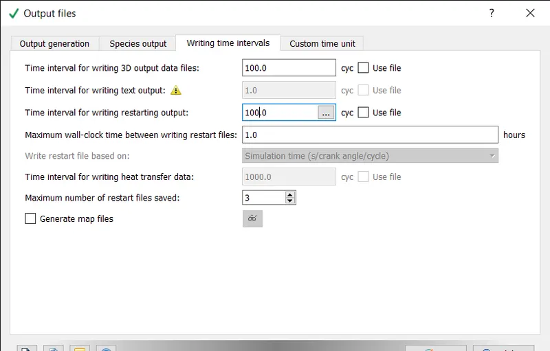
         The interval for writing 3d output data files and restarting outputs are defined.

          

• Exporting the input files to a folder
• Then the executable is pasted inside the folder
• The simulation is run in Cygwin.
• The postconvert executable is pasted in the output folder.
• The post conversion is done on Cygwin and converted into the type that paraview reads.
• The results are then post processed using paraview.

RESULT:

CASE 1:

VELOCITY = 680M/S AND SGS AS 0.01:

MESH:

 

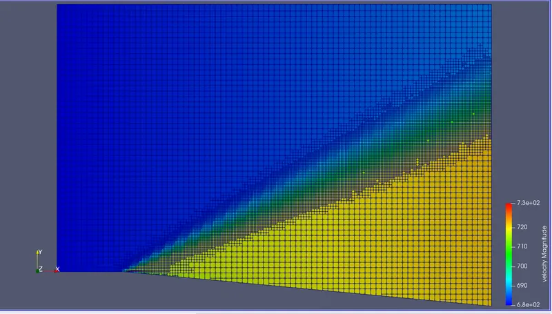
VELOCITY CONTOUR:

 

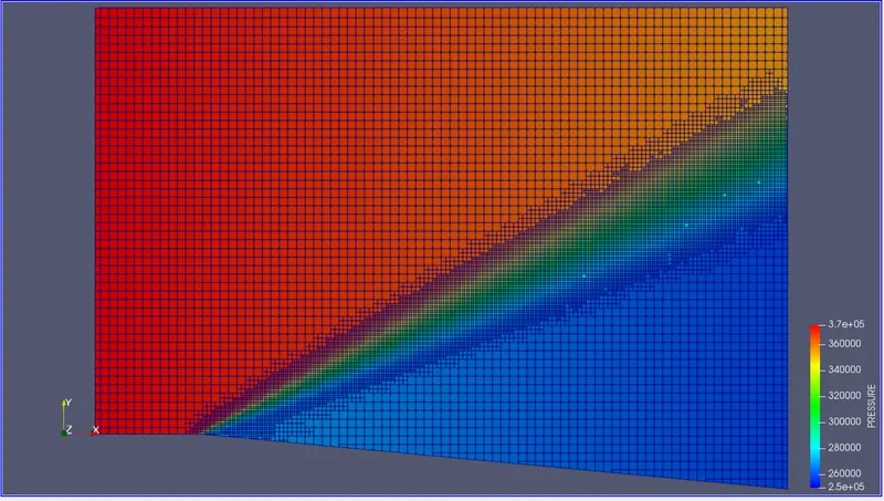
PRESSURE CONTOUR:

 

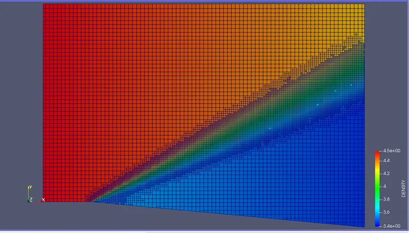
DENSITY:

 

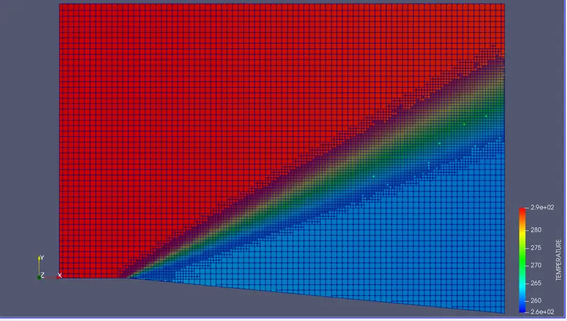
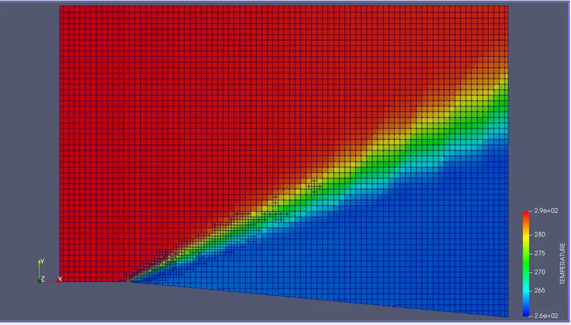
TEMPERATURE:

 

AVERAGE PRESSURE PROFILE:

 

AVERAGE VELOCITY PROFILE:

 

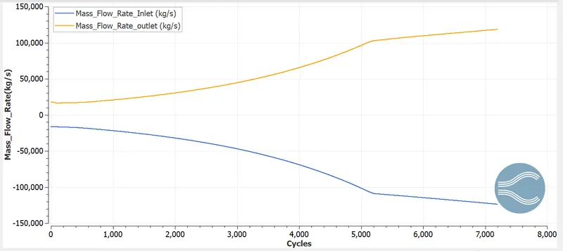
AVERAGE MASS FLOW RATE:

 

AVERAGE TEMPERATURE:

 

AVERAGE DENSITY:

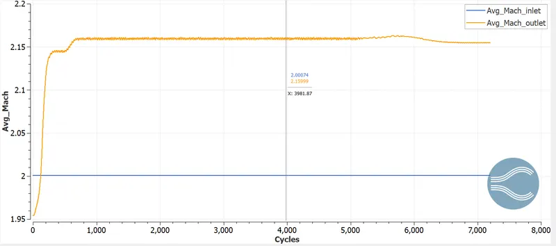
AVERAGE MACH NUMBER:

 

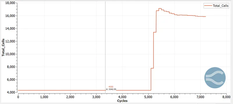
CELL COUNT:

 

 ANIMATION:

https://drive.google.com/file/d/1TjU8RTrfcDQ6UEIy4wEwFCciVoegWOPX/view?usp=sharing

CASE 2:

VELOCITY = 680M/S AND SGS AS 0.05:

MESH:

 

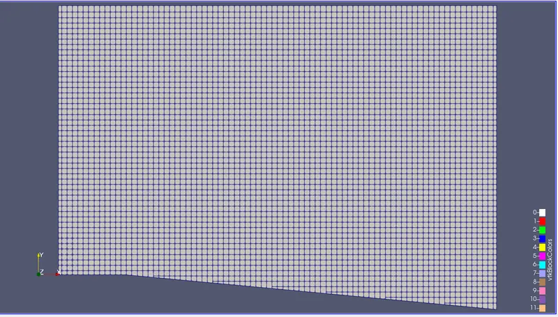
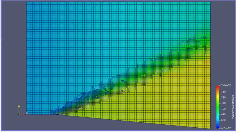
VELOCITY CONTOUR:

 

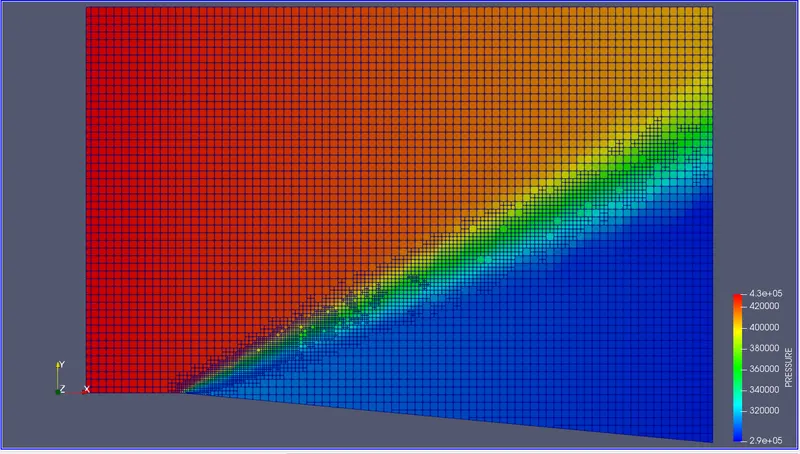
PRESSURE CONTOUR:

 

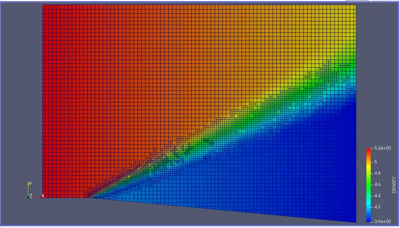
DENSITY:

 

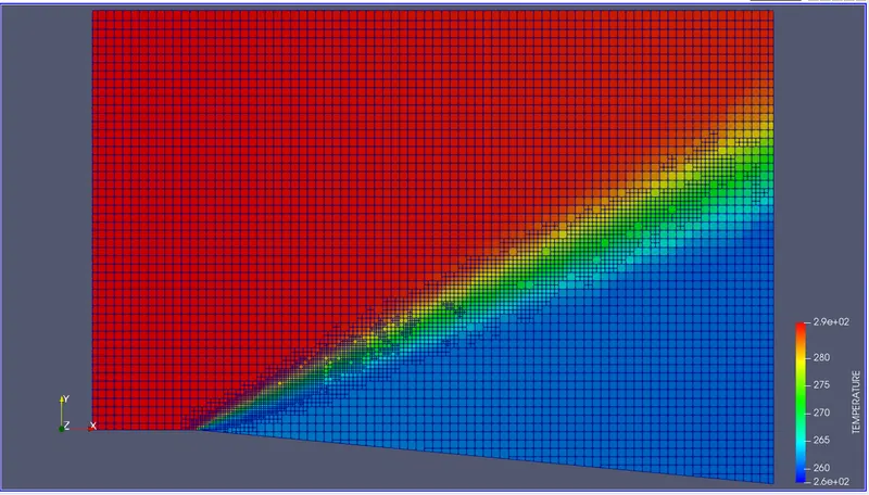
TEMPERATURE:

 

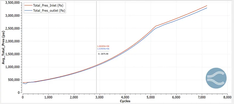
AVERAGE PRESSURE PROFILE:

 

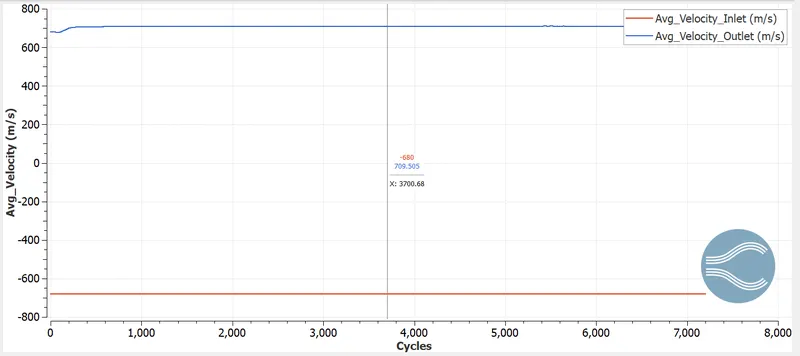
AVERAGE VELOCITY PROFILE:

 

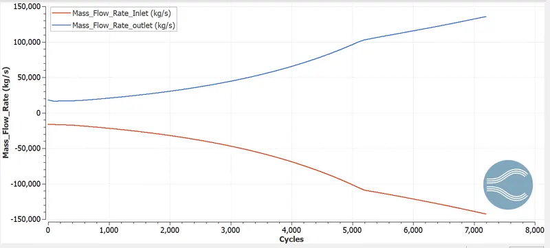
AVERAGE MASS FLOW RATE:

 

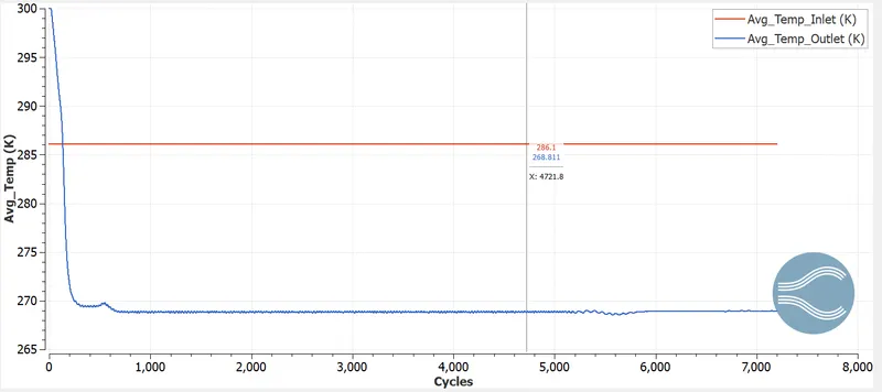
AVERAGE TEMPERATURE:

 

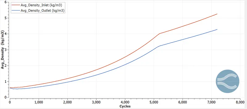
AVERAGE DENSITY:

 

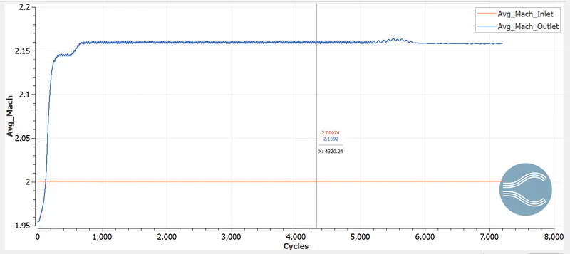
AVERAGE MACH NUMBER:

 

 

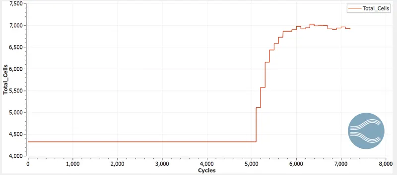
CELL COUNT:

 

ANIMATION:

 https://drive.google.com/file/d/1yVNjOXlEYu-0EAJBOL4XJMXFUx2Y8zIU/view?usp=sharing

CASE 3:

VELOCITY = 680M/S AND SGS AS 0.1:

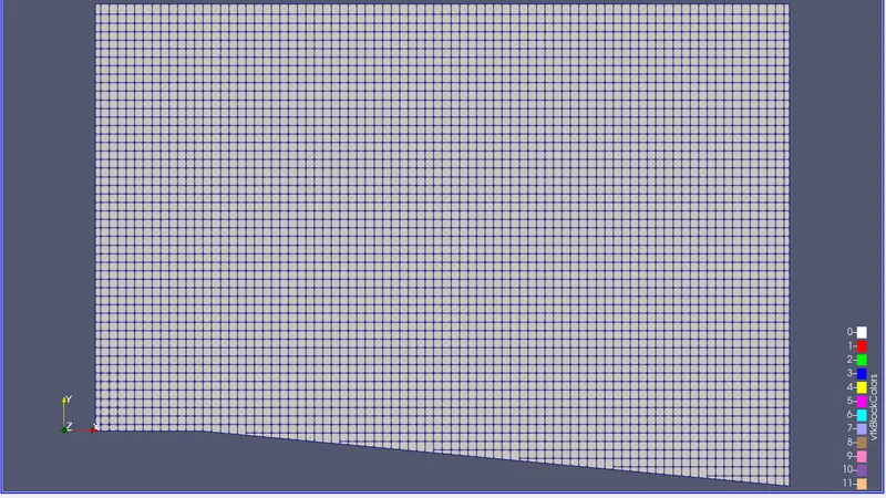
MESH:

 

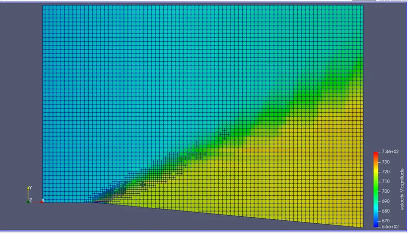
VELOCITY CONTOUR:

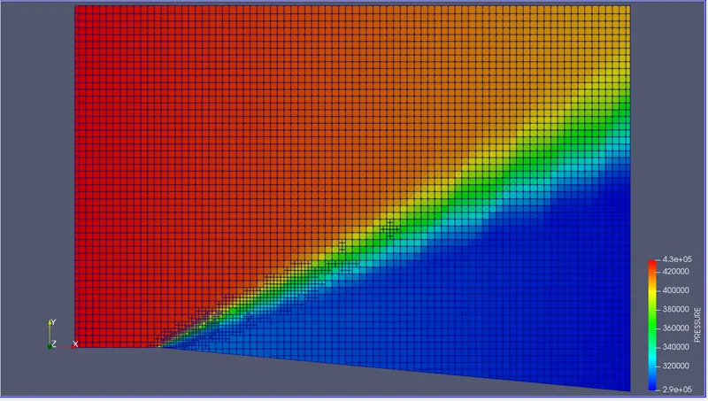
PRESSURE CONTOUR:

 

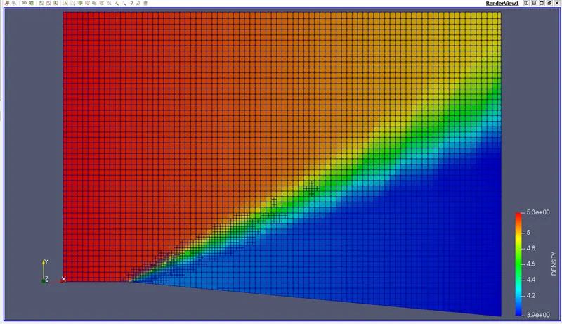
DENSITY:

 

TEMPERATURE:

 

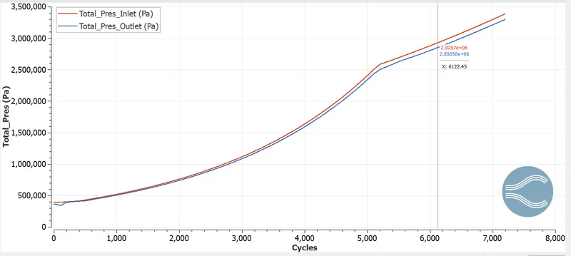
AVERAGE PRESSURE PROFILE:

 

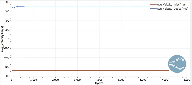
AVERAGE VELOCITY PROFILE:

 

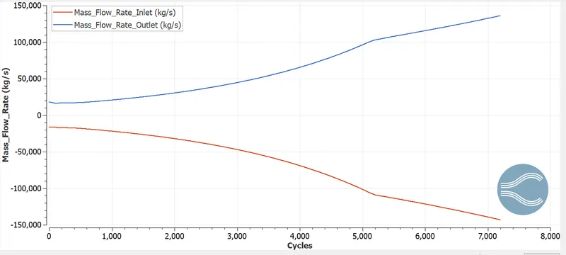
AVERAGE MASS FLOW RATE:

 

AVERAGE TEMPERATURE:

 

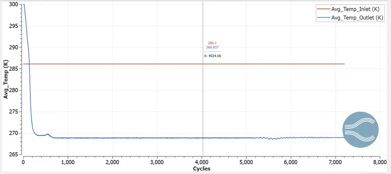
AVERAGE DENSITY:

 

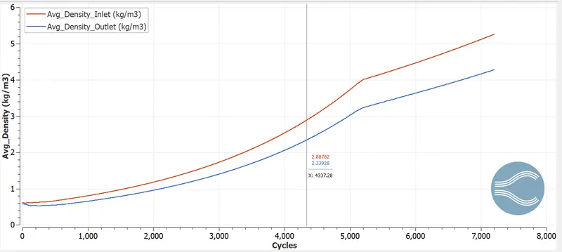
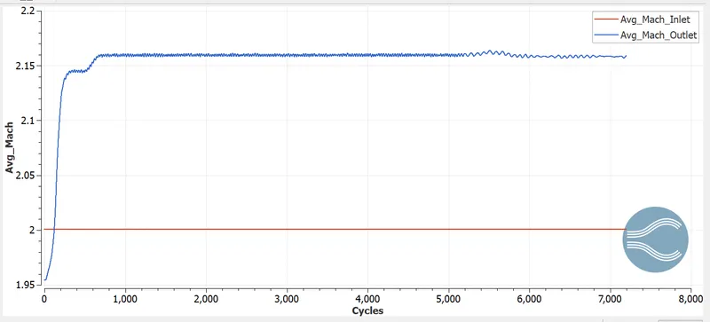
AVERAGE MACH NUMBER:

 

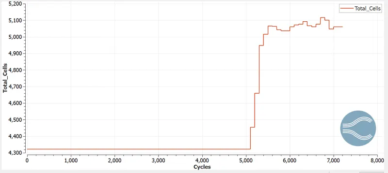
CELL COUNT:

 

 ANIMATION:

https://drive.google.com/file/d/1MQ0GwRSImizgqe3u4AZiOVbyzszeB5VC/view?usp=sharing

CASE 4:

VELOCITY = 100M/S AND SGS AS 0.05:

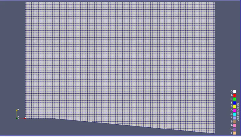
MESH:

 

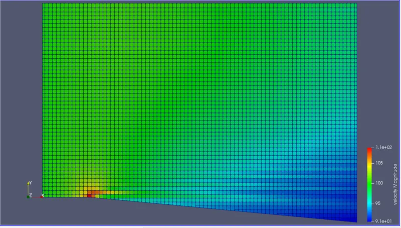
VELOCITY CONTOUR:

 

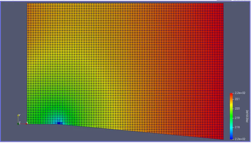
PRESSURE CONTOUR:

 

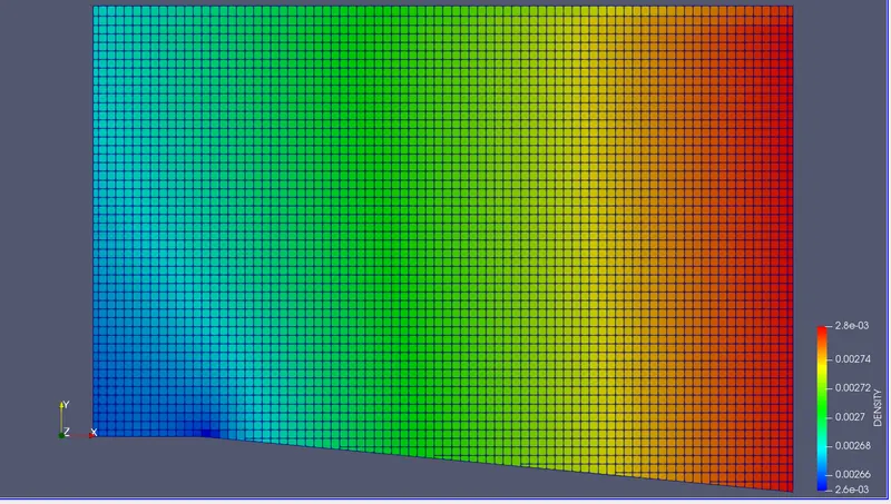
DENSITY:

 

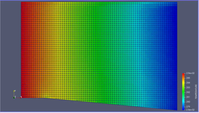
TEMPERATURE:

 

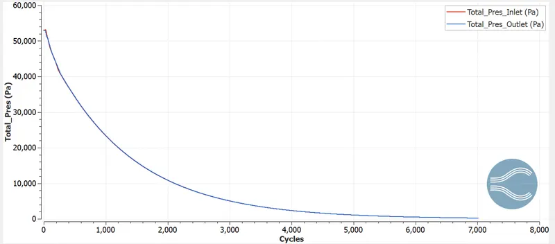
AVERAGE PRESSURE PROFILE:

 

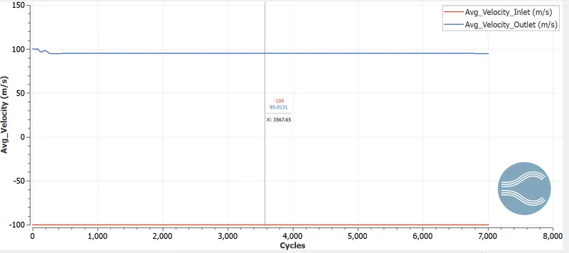
AVERAGE VELOCITY PROFILE:

 

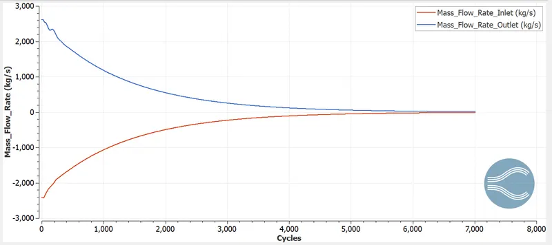
AVERAGE MASS FLOW RATE:

 

AVERAGE TEMPERATURE:

 

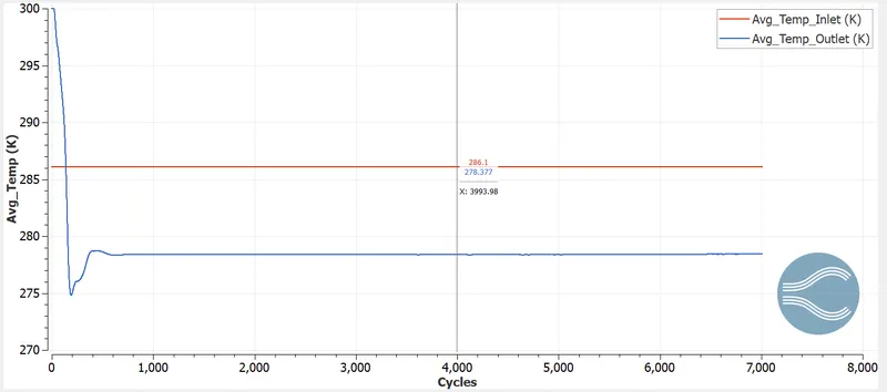
AVERAGE DENSITY:

 

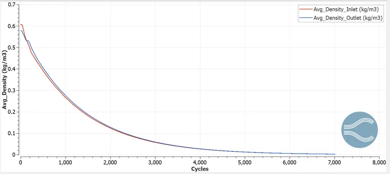
AVERAGE MACH NUMBER:

 

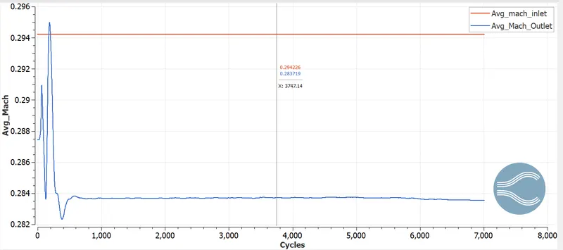
CELL COUNT:

 

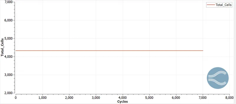
 ANIMATION:

https://drive.google.com/file/d/1bJ2EUTy3VsTmad5ir4pDdcxQzrt124qM/view?usp=sharing

OBSERVATION FROM ABOVE PLOTS:

EFFECT OF SGS:

• As SGS decreases, the total cell count increases. So that for small SGS parameter, AMR refines the mesh with more number of cells in and around the shock waves.
• For high SGS the mesh refinement area is very small whereas for small SGS the mesh refinement area is more. So for small SGS refinement spans from the sharp edge till the outlet boundary.

SUBSONIC VS SUPERSONIC FLOW COMPARISON:

• In supersonic flow, the Prandtl Mayer expansion fan is clearly visible and the mesh refinement is also visible in shock occurring regions.
• In subsonic flow, the Prandtl Mayer expansion fan is not visible and the mesh refinement is also not visible because there are no sudden fluctuations in parameters like pressure, temperature, velocity and density.
• The average Mach number increases from inlet to outlet in case of supersonic flow where as in subsonic flow it decreases.

CONCLUSION:

• The simulation of supersonic and subsonic flow through a duct was setup and run in converge CFD.
• The various contour plots are studied for different cases.
• The formation of shock waves and the effect of SGS on the shock location was studied.