Week 5: Prandtl Meyer Shock problem
Aim:
- To do Prandtl Meyer shock problem in CFD Converge and, In the Prandtl Meyer shock problem, look at the effect of SGS temperature value on cell count and the shock location.
Shock Waves:
-
It is a type of disturbance that propagates at a speed greater than the speed of sound in the medium. As a rule, like ordinary waves, shock waves carry energy and can propagate through a medium. Above all, we characterize a shock wave by a sudden, nearly discontinuous, change in pressure, temperature, and density of the medium.
Boundary Conditions in Shock Waves:
For solving the PDE's we need the sufficient and necessary boundary and initial conditions. If the model under study is steady-state we need only boundary conditions as no time derivative is involved. If it is transient model, we need the appropriate initial conditions of the domain as well.
Types of BC'S:
- Dirichet's Boundary Condition
- Neumann's Boundary Condition
- Robin's Boundary condition
- Mixed Boundary condition
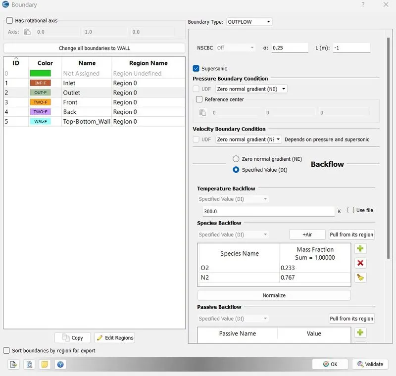
in this Shock wave problem we use Neymann's boundary condition, because for supersonic outlet the characteristic curves propogate outside the domain, long with the streamline. Hence, we have used zero normal gradient as the boundary conditio for pressure and velocity.
Procedure:
- Open CFD Converge and import the geometry and change the dimensions as required to minimize the number of cells.
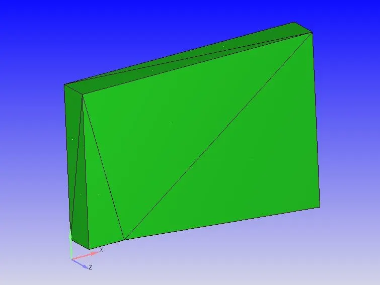
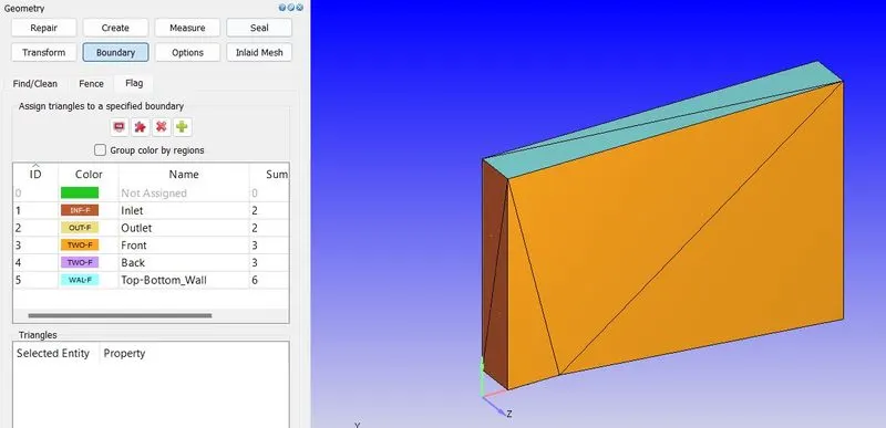
- Then assign the boundary flagging and check the normals.
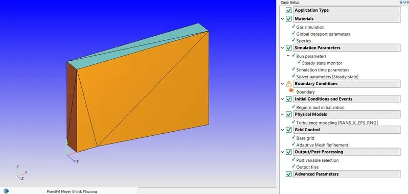
- After that set up cases one by one.
Case setup:
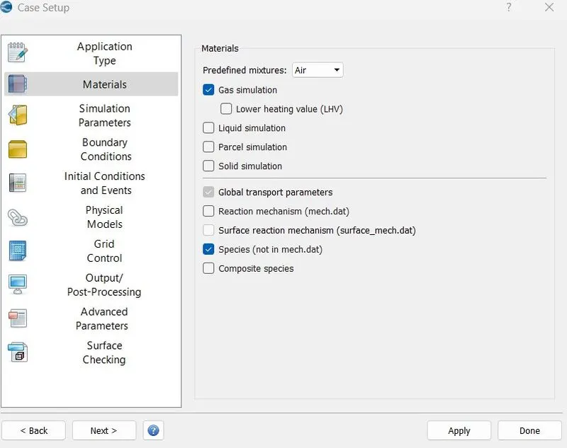
Materials:
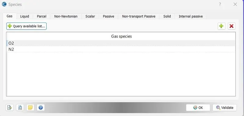
Species:
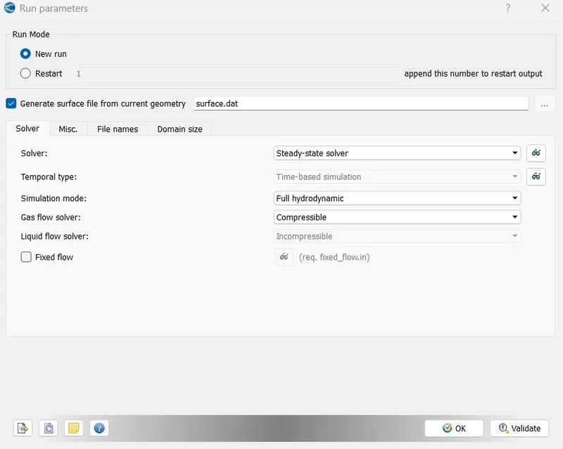
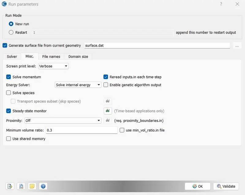
Run Parameter:
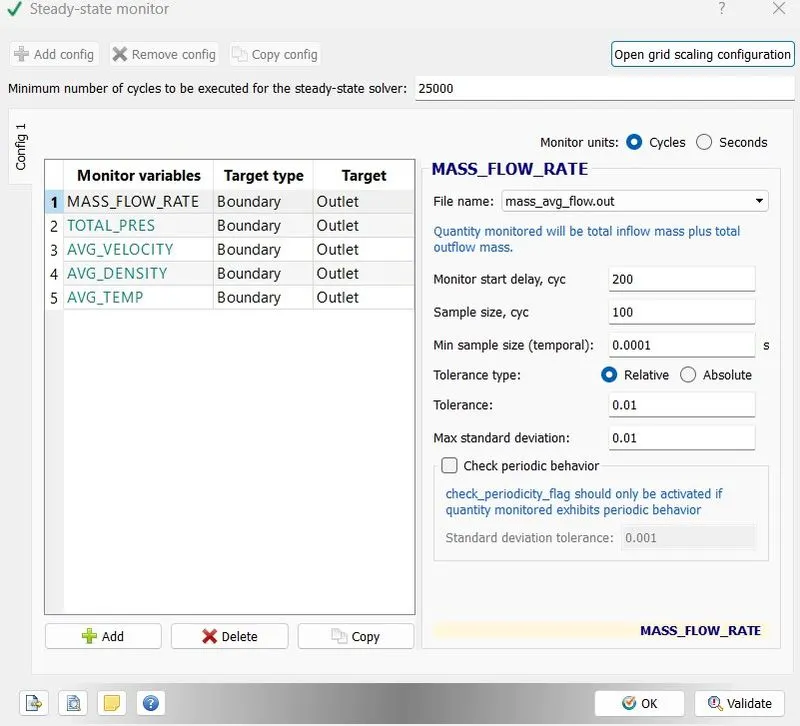
Steady state monitor:
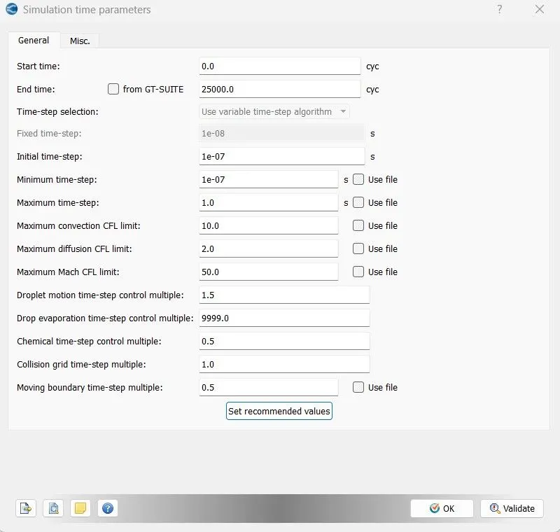
Simulation time parameter:
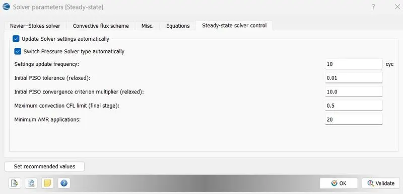
Solver parameter:
Boundary Conditions:
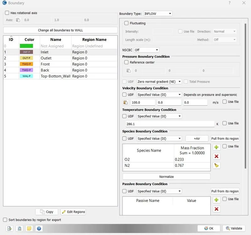
Inlet:
Outlet:
Front &back:
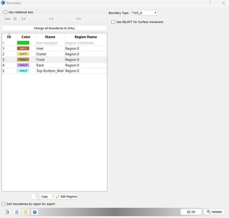
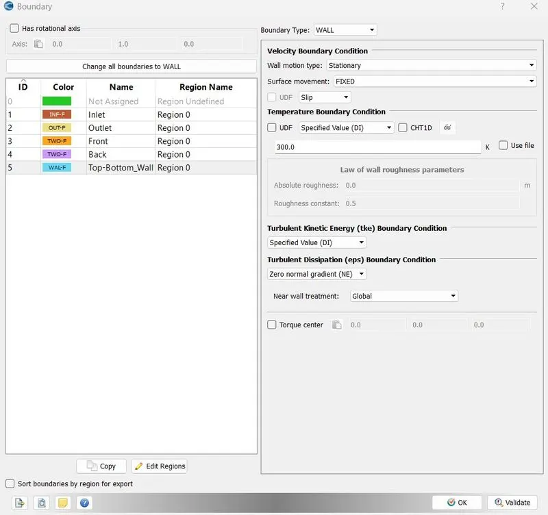
Top & Bottom:
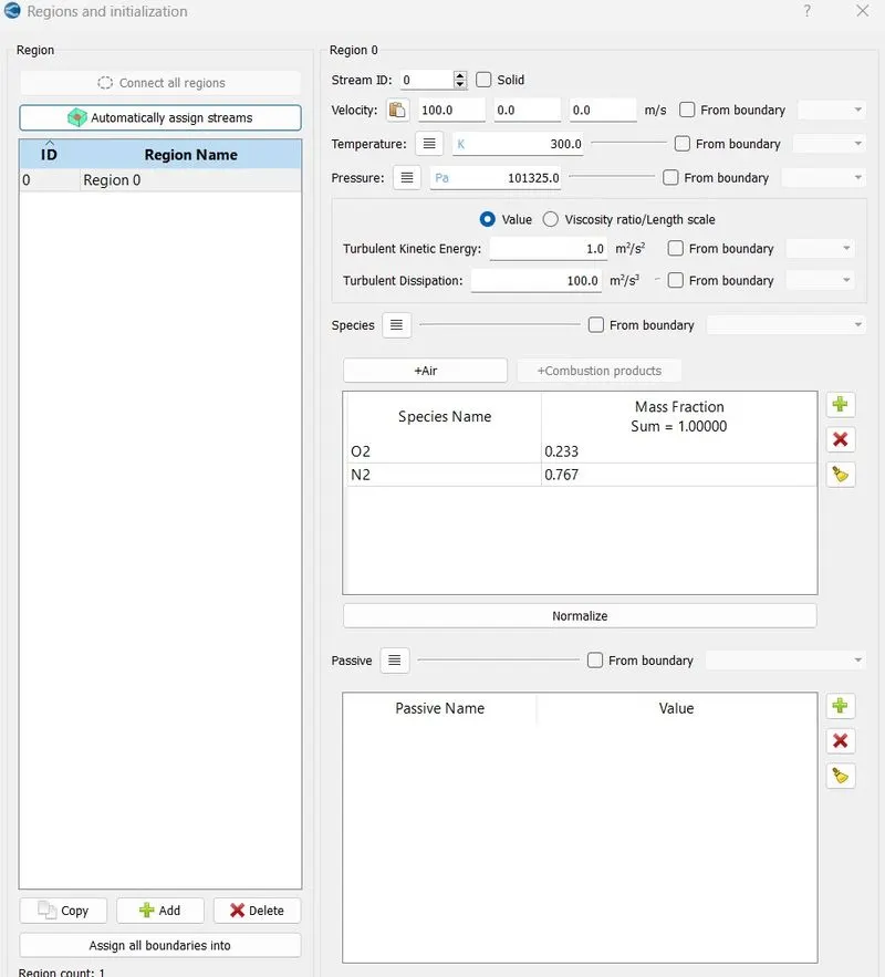
Region:
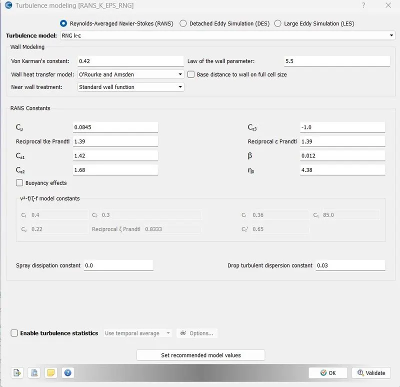
Turbulence modeling
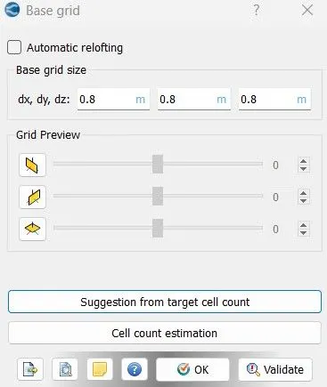
Base Grid:
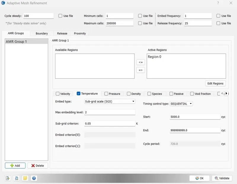
Adaptive Mesh Refinement:
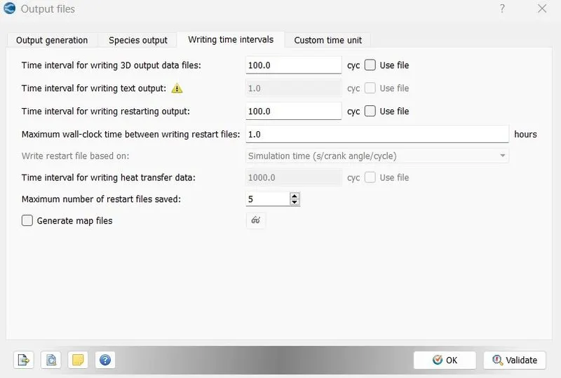
Output Files:
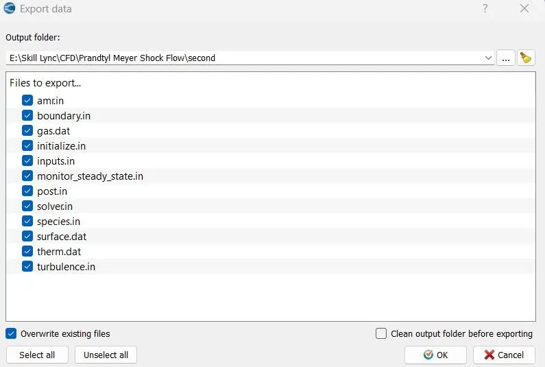
- After setting up all cases then export the input files to the required directory
Export:
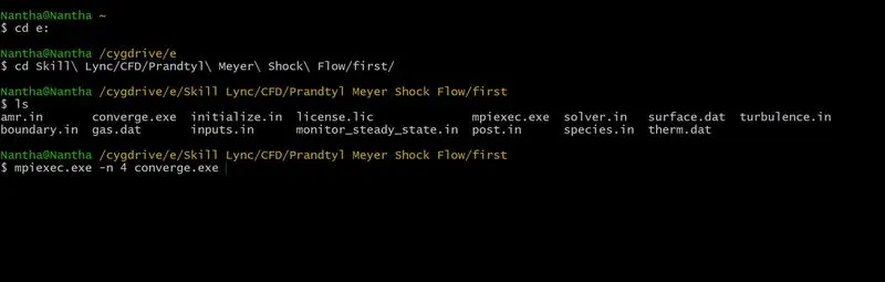
- After export the input files, run the simulation using Cygwin.
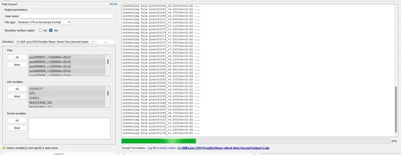
- Then Post convert the output files so that we can anlyse the result plots.
- Create average velocity plot, pressure plot and average temperature plot in converge and paraview and also create a required animations.
- Repeat the same process with different cases so that we can understand the differances.
Cases:
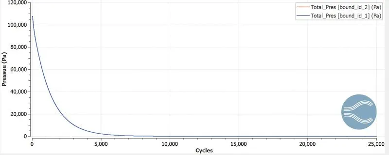
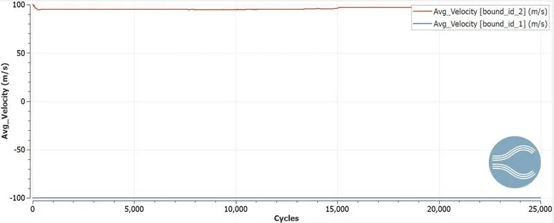
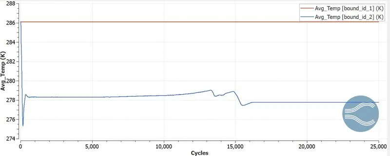
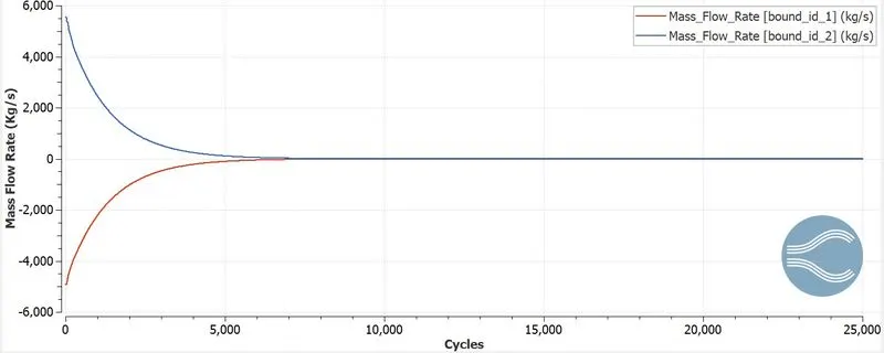
1. Velocity = 100 m/s and SGS Temperature sub grid criteria = 0.05
2.Velocity = 680 m/s and SGS Temperature sub grid criteria = 0.3
Results:
Case- 1
Velocity = 100 m/s and SGS Temperature sub grid criteria = 0.05
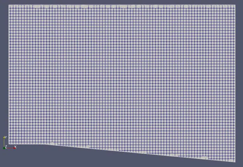
Mesh:
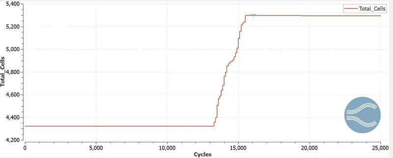
Total Cell Count:
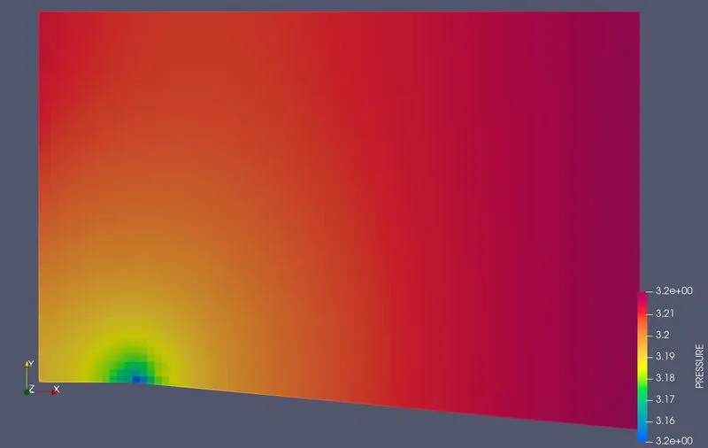
Pressure Plot:
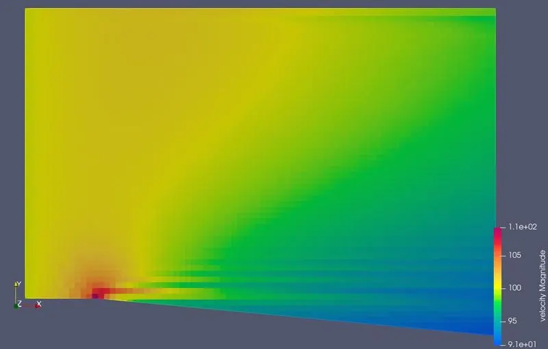
Velocity Plot:
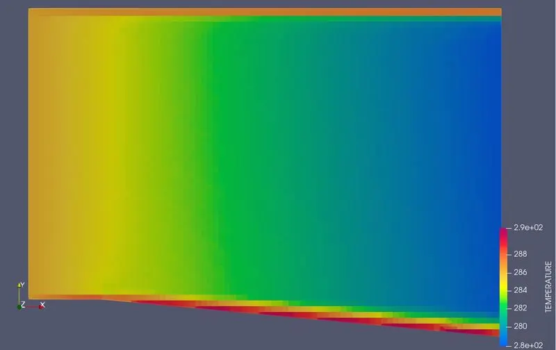
Temperature Plot:
Mass Flow Rate:
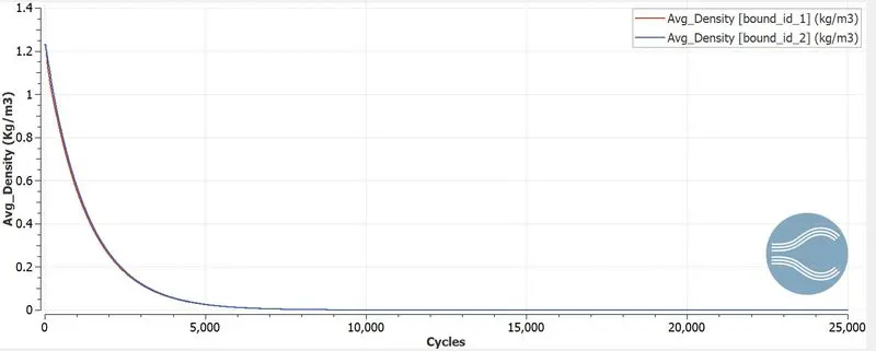
Density Plot:
Pressure Contour:
Velocity Contour:
Temperature Contour:
Density Contour:
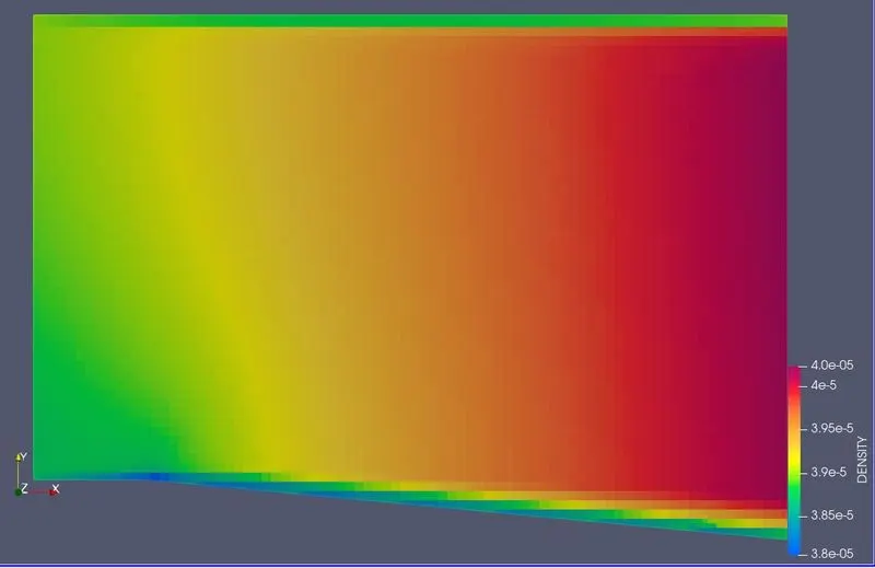
Animations:
Pressure:
Velocity:
Temperature:
Case- 2
Velocity = 680 m/s and SGS Temperature sub grid criteria = 0.3
Mesh:
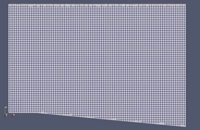
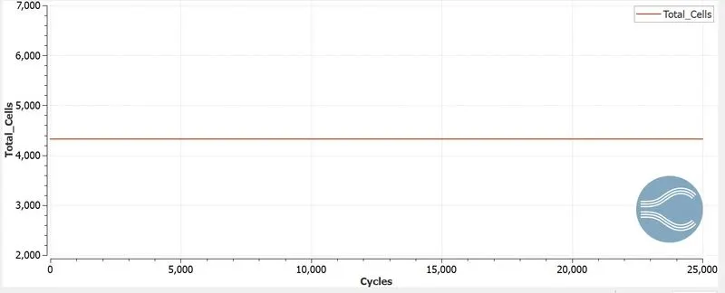
Total Cell Count:
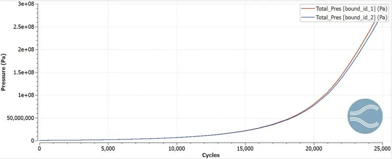
Pressure Plot:
Velocity Plot:
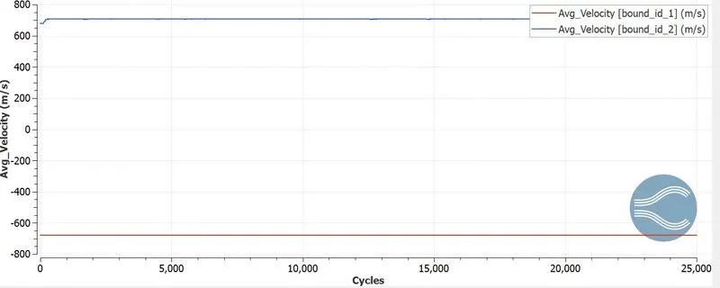
Temperature Plot:
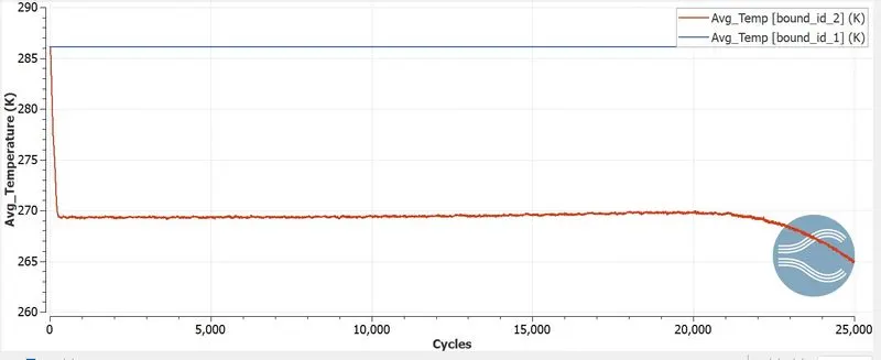
Mass Flow Rate:
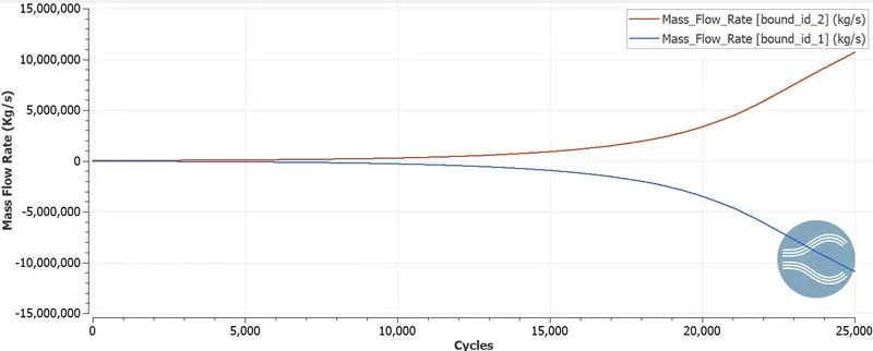
Density Plot:
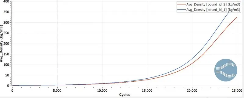
Pressure Contour:
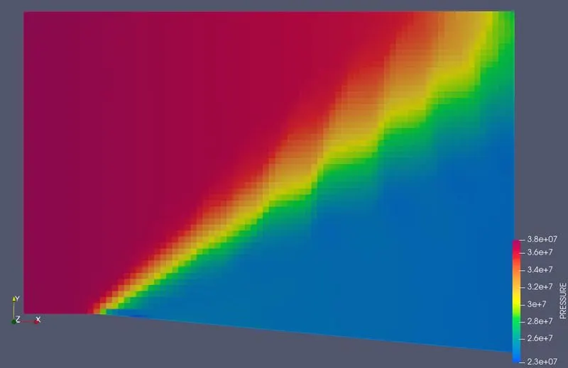
Velocity Contour:
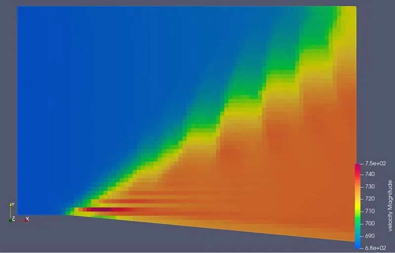
Temperature Contour:
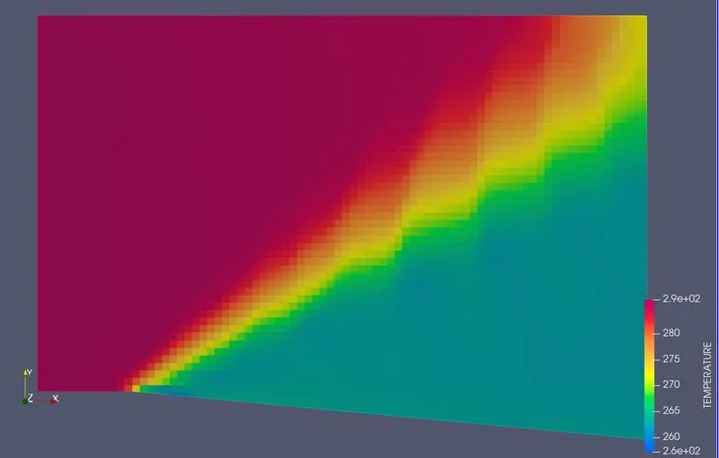
Density Contour:
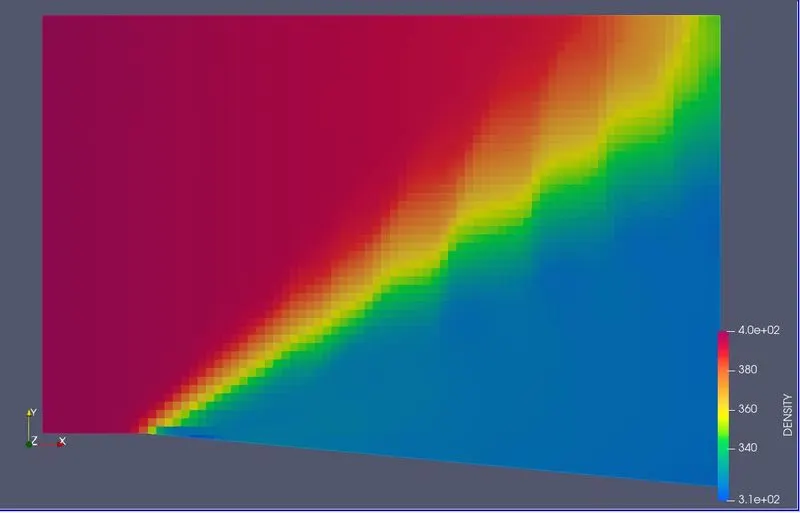
Animations:
Pressure:
Velocity:
Temperature:
Conclusion:
- The Cell counts increases when we discrease the temperature sub grid scale criteria.
- By increasing the cell count and decreasing the SGS criteria we are able to capture accurate shock waves.