Prandtl Meyer Expansion fan shock problem simulation with AMR Technique.

PRANDTL MEYER EXPANSION FAN.

Aim:-

The Prandtl Meyer shock flow is analyzed with a subsonic and supersonic wave and the effect of SGS parameters in the problem.

Objective:-

• Run the Simulation with Subsonic(100m/s) and Supersonic(678m/s) waves.
• Varying the Sub-grid Criteria value in Adaptive mesh refinement to look at the effect of SGS temperature.
• Do a literature search on what BCs are typically used for shock flow problems.
• What is a shock wave? Describe the Physics behind shock waves.
• Show the mesh generation using Paraview.

INTRODUCTION

At the molecular level fluid particles travel in a continuum, when an obstruction is suddenly introduced in the flow, something interesting happens. The particle in front of it slows down instantaneously creating an increase in local pressure. Since the fluid is continuam the information of whatever happens in one place is transmitted to other regions in the form of pressure waves. This pressure wave then causes the oncoming fluid to adjust its properties.

Sound travel through the medium in the form of compression and rarefaction. But the information propagation in fluid happens through the acoustics waves which travel at the speed of sound.

When the fluid particles are traveling faster than the speed of sound, and since the information transfer can not happen faster than the speed of sound, the oncoming particles don't have any information about the coming obstruction in front until they reach it. The moment they reach it, the extreme collision of particles with themselves and the object occurs, manifesting as a shockwave.

Mach Number -
* Mach number is a dimensionless number which is very important while studying the shocks. Mach number is the ratio of the velocity of the fluid(μ">μ) to the velocity of sound in that medium(a). So clearly if the Mach number is greater than 1, this means fluid is traveling faster than the speed of sound meaning, there is no time for the information to propagate, these flows are called supersonic flows.

SHOCKWAVE

In physics, a shock wave (also spelled shockwave), or shock, is a type of propagating disturbance that moves faster than the local speed of sound in the medium. Like an ordinary wave, a shock wave carries energy and can propagate through a medium but is characterized by an abrupt, nearly discontinuous, change in pressure, temperature, and density of the medium.

When the speed of the object exceeds the speed of the sound, the wavefronts lag behind the source in a cone-shaped region with the source at the vertex. The edge of the cone forms a supersonic wave with a large amplitude called a "shock wave". when a shock wave reaches an observer a "sonic boom" is heard.

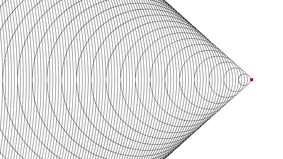
In a shock wave, the properties of the fluid (density, pressure, temperature, flow velocity, Mach number) change almost instantaneously.

For comparison, in supersonic flows, additional increased expansion may be achieved through an expansion fan, also known as a prandtl-Mayer expansion fan. The accompanying expansion wave may approach and eventually collide and recombine with the shock wave, creating a process of destructive interference. The sonic boom associated with the passage of a supersonic aircraft is a type of sound wave produced by constructive interference.

Unlike solitons (another kind of nonlinear wave), the energy and speed of a shock wave alone dissipate relatively quickly with distance. Energy is preserved when a shock wave passes through matter, but entropy increases. This change in the matter's properties manifests itself as a decrease in the energy which can be extracted as work, and as a drag force on supersonic objects; shock waves are strong.

A moving shock is called a shock wave which is very thin in the order of 200 nanometers and it's under this region where
fluid undergoes a sudden change of properties. The Mach number decreases across the shockwave, along with the sudden rise in pressure, density, and temperature. Shockwave is also an irreversible process because of the extreme reactions produced by the collision of the particles.

In some aerospace applications, an engineer always tries to reduce the shock as it causes vibrations and an increase in drag.
Even in commercial aircraft which never go supersonic, there are regions over the wing where the flow can locally go supersonic, this is the exact region why commercial airplanes have swept-back wings. When air now flows over the wing, it sees a thinner wing because only a component of the velocity is perpendicular to it and doesn't accelerate to supersonic speeds.

When a stationary object emits sound waves at a certain frequency, the waves are generally spherical in nature and travel at the speed of sound. The moment an object starts moving, the sound waves in front of it compressed increasing the apparent frequency, and the ones behind elongated decrease the apparent frequency, this effect is known as the Doppler effect. When the object travels faster than the speed of sound, the sound waves that are emitted from a cone are known as the Mach cone.

Shock waves can be:

Normal

At 90° (perpendicular) to the shock medium's flow direction.

When the flow is not turned at all, the resulting shock is called a normal shock since it forms perpendicular to the surface.
Normal shocks occur when there is a change in the flow area and similar to bow shocks they change the flow from supersonic to subsonic and similar to oblique shocks, they are also attached to the body.
Normal shocks often form on the wing's upper surface, because the flow speeds up enough locally to go supersonic. Since normal shocks also have drag, high-speed aircraft often have swept wings so these normal shocks behave like oblique shocks, and airspeed is maintained.

Oblique Shockwave

At an angle to the direction of flow.

Now as the object becomes more streamlined, eventually more pointed the shock wave will too until it hits a critical point, where bow shock becomes an attached oblique shock. The critical point depends on the speed of the flow and the angle of the cone. Aircraft designers want to avoid bow shocks at all costs since they provide a detrimental amount of drag. Oblique shocks are formed when the supersonic flow is rapidly redirected onto itself. This flow has little effect on drag because they don't slow down the air, they speed it up.

Bow/Detached Shockwave

Occurs upstream of the front (bow) of a blunt object when the upstream flow velocity exceeds Mach 1.

This type of form in front of the ball is known as bow shock or detached shock. It is special that it does not connect to the ball in any way. It is also very complicated to study since it very much depends on the geometry of the object. But in general bow shocks will form only with blunt objects.

Expansion Waves -
Expansion shocks are formed when the supersonic flow suddenly turns around the corner as shown in the figure. It is the opposite of oblique waves, where waves are turned onto themselves, whereas in this waves are turned away from themselves. These waves are also known as Prandtl Meyer expansion fan which is made up of an infinite amount of oblique waves.

Some other terms:

• Shock front: The boundary over which the physical conditions undergo an abrupt change because of a shock wave.
• Contact front: In a shock wave caused by a driver gas (for example the "impact" of a high explosive on the surrounding air), the boundary between the driver (explosive products) and the driven (air) gases. The Contact Front trails the Shock Front.

NEED INITIAL CONDITIONS AND BOUNDARY CONDITIONS
Consider an example of a pipe whose one end is placed at a heating source i.e. heat is continuously being added at one end.
To know the temperature distribution along the pipe and want to find the scalar temperature field in space and time, initial and boundary conditions are needed to solve the respective P.D.E.

TYPES OF BOUNDARY CONDITIONS -

There are 5 types of boundary conditions -
1. Dirichlet boundary condition
2. Neumann boundary condition
3. Robin's boundary condition
4. Mixed boundary condition
5. Cauchy boundary condition

Boundary Conditions:

In CFD, Boundary Conditions (BC) are equally important as the governing equations, even if most textbooks deal predominantly with the governing equations only. From a mathematical point of view, BCs are inherently linked with PDEs. A PDE must have BCs to obtain a unique solution. In CFD, the various solutions to the same governing equations are distinguished by the BCS. In other words, the flow over a car differs from the flow over a Space Shuttle exactly because of the different BCs applied.

Specifying of wrong boundary conditions in the CFD imposing the solution to blown up or given a wrong Convergence solution.

Dirichlet boundary Conditions:

In mathematics, a Dirichlet problem is the problem of finding a function that solves a specified partial differential equation (PDE) in the interior of a given region that takes prescribed values on the boundary of the region.

The value of the dependent variable is specified on the boundary.

y=f

For example, if one end of an iron rod is held at absolute zero, then the value of the problem would be known at that point in space

Neumann boundary conditions:

A boundary condition that specifies the value of the normal derivative of the function is a Neumann Boundary Condition or second-type boundary condition.

The normal derivative of the dependent variable is specified on the boundary.

dy/dx = f

For example, if there is a heater at one end of an iron rod, then energy would be added at a constant rate but the actual temperature would not be known.

Robin boundary conditions:

Robin boundary conditions are a weighted combination of Dirichlet boundary conditions and Neumann boundary conditions. This contrasts with mixed boundary conditions, which are boundary conditions of different types specified on different subsets of the boundary. Robin boundary conditions are also called impedance boundary conditions, from their application in electromagnetic problems, or convective boundary conditions, from their application in heat transfer problems

It is imposed on an ordinary or a partial differential equation, it is a specification of a linear combination of the values of a function and the values of its derivative on the boundary of the domain.

Cauchy Boundary Condition:

The Cauchy Boundary Conditions augments an ordinary differential equation or a partial differential equation with conditions that the solution must satisfy on the boundary; ideally so to ensure that a unique solution exists. A Cauchy boundary condition specifies both the function value and normal derivative on the boundary of the domain. This corresponds to imposing both a Dirichlet Boundary Condition and a Neumann boundary condition.

Cauchy boundary conditions are simple and common in second-order ordinary differential equations.

Mixed boundary condition

Mixed boundary conditions refer to the case in which Dirichlet boundary conditions are prescribed in some parts of the boundary while Neumann boundary conditions exist in others.

Boundary conditions Used for shock flow problems -

* For compressible flows, the inlet conditions are generally known hence, the constant value is given at the domain i.e Dirichlet boundary condition. In shock flow problems outlet conditions are not known because, the shock causes huge variation in flow properties, which leads to a gradient across the normal surface. This can be extrapolated from the inlet conditions and the basic properties of the flow by defining the zero normal gradients i.e. Neumann boundary condition at the outlet.

Prandtl Mayer Shock

A supersonic expansion fan, technically known as Prandtl–Meyer expansion fan, a two-dimensional simple wave, is a centered expansion process that occurs when a supersonic flow turns around a convex corner. The fan consists of an infinite number of Mach waves, diverging from a sharp corner. When a flow turns around a smooth and circular corner, these waves can be extended backward to meet at a point.

Each wave in the expansion fan turns the flow gradually (in small steps). It is physically impossible for the flow to turn through a single "shock" wave because this would violate the second law of thermodynamics.

Across the expansion fan, the flow accelerates (velocity increases) and the Mach number increases, while the static pressure, temperature, and density decrease. Since the process is isentropic, the stagnation properties (e.g. the total pressure and total temperature) remain constant across the fan.

The theory was described by Theodor Mayer in his thesis dissertation in 1908, along with his advisor Ludwig Prandtl, who had already discussed the problem a year before.

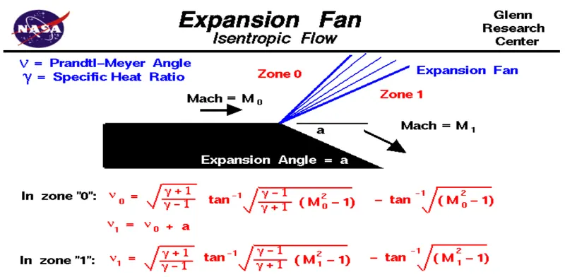
When a supersonic flow encounters a convex corner, it forms an expansion fan, which consists of an infinite number of expansion waves centered at the corner. The above figure shows one such ideal expansion fan.

As opposed to the flow encountering an inclined obstruction and forming an oblique shock, the flow expands around a convex corner and forms an expansion fan through a series of isentropic Mach waves. The expansion "fan" is composed of Mach waves that span from the initial Mach angle to the final Mach angle. Flow can expand around either a sharp or rounded corner equally, as the increase in Mach number is proportional to only the convex angle of the passage (δ). The expansion corner that produces the Prandtl-Meyer fan can be sharp (as illustrated in the figure) or rounded. If the total turning angle is the same, then the P-M flow solution is also the same.

The Prandtl-Meyer expansion can be seen as the physical explanation of the operation of the Laval nozzle. The contour of the nozzle creates a smooth and continuous series of Prandtl-Meyer expansion waves.

The expansion fan consists of an infinite number of expansion waves or Mach lines. The first Mach line is at an angle `mu1=arcsin(1/(M1))` concerning the flow direction, and the last Mach line is at an angle `mu2=arcsin(1/(M2))`concerning the final flow direction. Since the flow turns in small angles and the changes across each expansion wave are small, the whole process is isentropic. This simplifies the calculations of the flow properties significantly. Since the flow is isentropic, the stagnation properties like stagnation pressure `P0'>P0`, stagnation temperature `T0'>T0` and stagnation density (`ρ0>ρ0` remain constant.

Effect of SGS parameter on shock location.

Use Adaptive Mesh Refinement (AMR) to automatically refine the grid based on fluctuating and moving conditions such as temperature or velocity. This feature may be used to obtain a refined grid in flow regions of interest allowing complex phenomena, such as flame propagation or high-velocity flow, without unnecessarily slowing the simulation with a globally refined grid.

There are two types of AMR: sub-grid scale (SGS)-based and value-based. The AMR type and criteria should be chosen such that a higher grid resolution (embedding) is added where the flow field is most under-resolved, where the sub-grid field is the largest (i.e., where the curvature [gradient] of a specified field variable is the highest), or where a variable satisfies
the embed criteria. The default AMR method in CONVERGE estimates the magnitude of the sub-grid field to determine where CONVERGE will add embedding.

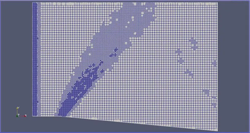
The adaptive mesh refinement technique was used because the region where the shock would occur require the mesh to be refined locally. The mesh in the other regions has the same size as the base grid size whereas in the region where shock occurs finer cells are used. Temperature-based mesh refinement was used that would monitor curvature in temperature. Temperature-based mesh refinement was used that would monitor the gradient in temperature. Gradient means `(del^2T)/(delx^2)`. When the temperature is greater than a particular value defined by the user the mesh is refined. In the first run, the SGS is taken as 0.05K. When the subgrid is greater than 0.05K, the mesh would refine.

----------------------------------------------------------------------------------------------------

PROCEDURE :

Simulation Process

Part 1 - Subsonic condition (velocity 100 m/s)

• SGS temperature of 0.05 K
• SGS temperature of 0.025 K
• SGS temperature of 0.01 K

Part 2 - Supersonic condition (velocity 678 m/s)

• SGS temperature of 0.05 K
• SGS temperature of 0.025 K
• SGS temperature of 0.01 K

To simulate steady-state flow over a throttle body the procedure is established:

Geometry Creation --> Case Setup --> Solution --> Post Processing

Geometry Creation :

Launch Converge and start a new project.
Drag and drop the .stl model in converge.

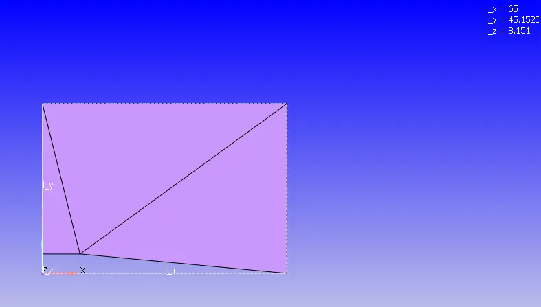
In converge, geometries are represented as triangles. So we need to group these triangles to create boundaries. This is a fundamental step in Converge.
Geometery => Boundary => Flag => click on add and add 3 boundaries => rename first boundary as inlet => using by angle triangle selection,select front face triangles => apply.
Similarly flag outlet, top, bottom, front and back.

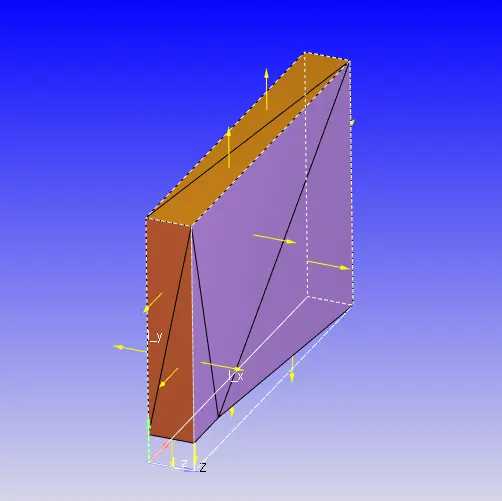
As our flow is internal, we want all the normals to point to the fluid domain. To do that,
click on normal toggle => transform => normal => click on triangle with outside pointing normal => apply

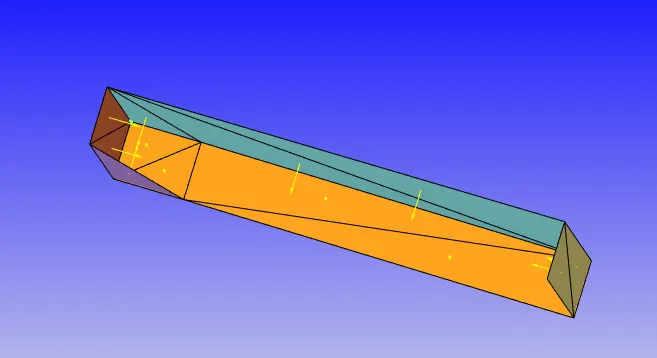
Make sure that geometry is clean,
Diagnosis => find => no errors.

Case Setup :

Click on Begin Case Setup => General Flow => Done.
Our working fluid will be air.
Materials => Predefined mixture => Air => uncheck reaction mechanism => check species => Apply & Done.

Keep default global transport parameters.

In species add oxygen and nitrogen.

Steady State flow is required to simulate if the final output is important.

In the solver time parameter, we only choose the pressure-based solver and retain the remaining sets.

a] Run Parameters => Solver => select solver type steady state solver => simulation mode full hydrodynamic => Gas flow solver compressible.
b] In Misc => check steady state monitor => uncheck use shared memory.

In converge it is mandatory in steady-state simulation to define monitor points, so that solver knows when to terminate the
simulation in order to save computation time.
Steady State Monitor => Add Config. => then add average velocity, total pressure, and mass flow rate.

The monitor start display is a parameter that ensures that the simulation runs for a certain number of cycles before the variable can be monitored. This is especially useful in transient simulations when you want the solution to run for a particular amount of time before checking for convergence if the steady state results are also required.

Sample size denotes the number of cycles or seconds over which the variable is checked to see if the solution has converged. The solution is said to converge when the average change over multiple iterations is less than the tolerance value. The tolerance value can be changed based on the problem and the level of accuracy required.

We need to define the minimum number of cycles that are required for the simulation to run before terminating and set it to 1000 cycles.

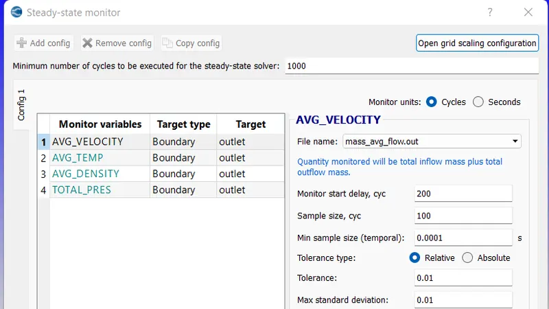
Simulation time parameters =>

Start Time - 0 cycles
End Time - 25000 cycles
Initial Time Step - 1e-7 sec.
Minimum Time Step - 1e-7 sec.
Maximum time step - 1 sec.
Maximum Convection CFL limit - 1.0.

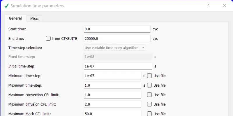
Initialization

Now before setting the boundaries, set the initial region and set initial pressure, and define air species. This region will be assigned to each boundary. For the subsonic case, velocity is 100m/s and for the supersonic case, velocity is 678m/s.

----------------------------------------------------------------------------------------------------------------

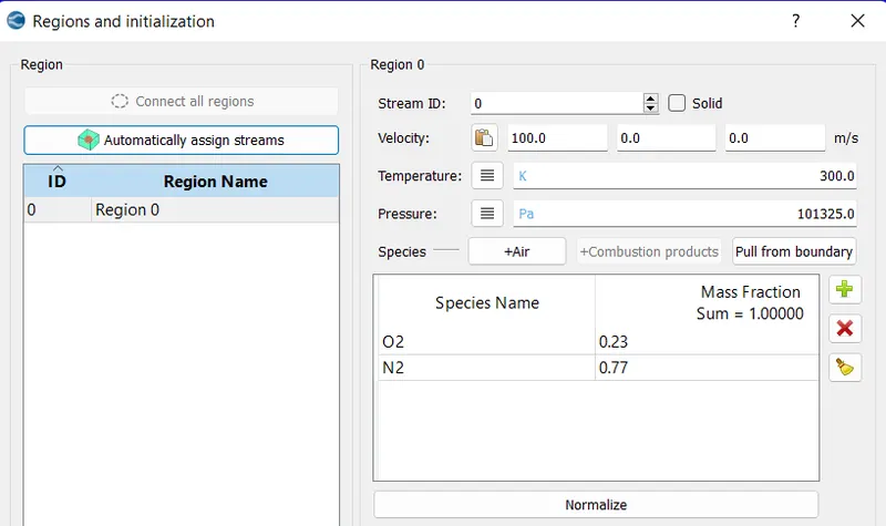
Boundary Conditions

Inlet -

• The boundary type is INFLOW
• Pressure Boundary Conditions- Zero Normal Gradient (Neumann Boundary)
• Velocity Boundary Conditions-100 m /sec and the velocity of sound is 340 m/sec

Mach number =Velocity of the object / velocity of the sound =100/ 340 = 0.294

• The temperature should be 286.1k and
• Add species 02=0.23 N2=0.77

Outlet

• The boundary type is OUTFLOW
• Pressure Boundary Conditions- Zero Normal Gradient (Neumann Boundary)
• Velocity Boundary Conditions- Zero Normal Gradient (Neumann Boundary)
• The temperature should be 300 k and
• Add species 02=0.23 N2=0.77

Front, Back, Top and Bottom Boundary Conditions:

• For the Front wall boundary should be the 2D wall type.
• For the Back wall Boundary type should be the 2D wall type.
• For the Top and Bottom wall the boundary type is WALL type with the slip condition as a boundary condition and temperature should be 300K.

---------------------------------------------------------------------------------------------------------------------------

MESHING

Grid Control:

• Element size dx=dy=dz=0.8 m

Adaptive Mesh Refinement:

In numerical analysis, adaptive mesh refinement (AMR) is a method of adapting the accuracy of a solution within certain sensitive or turbulent regions of simulation, dynamically and during the time the solution is being calculated. When solutions are calculated numerically, they are often limited to pre-determined quantified grids as in the Cartesian plane which constitute the computational grid, or mesh. Many problems in numerical analysis, however, do not require a uniform precision in the numerical grids used for graph plotting or computational simulation, and would be better suited if specific areas of graphs which needed precision could be refined in quantification only in the regions requiring the added precision. Adaptive mesh refinement provides such a dynamic programming environment for adapting the precision of the numerical computation based on the requirements of a computation problem in specific areas of multi-dimensional graphs which need precision while leaving the other regions of the multi-dimensional graphs at lower levels of precision and resolution.

In our case we need more refinement of mesh at the shock were occur in that region we need more refinement of mesh in that area and the remaining should be the normal grid size mesh.

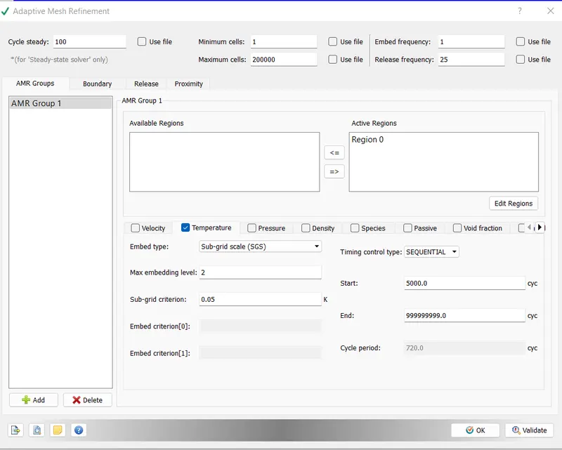
In converge we have the different methods which are used for the Adaptive Mesh Refinement Right now we are using the Temperature based Sub-Grid-Criterion method with the 2 embedded layers. Thus the converge helps the curvature of temperature property provided in AMR and starts the refining of the mesh for the temperature curvature by checking the values provided in the SGS where the valve is greater than the provided valve in SGS.This property helps us in the cost of computational domain and saves the time by not doing the unnnecessary meshing for the entire domain.

• In the Grid control enable the Adaptive Mesh Refinement
• In Adapative Mesh Refinement the volumetric region is changed from the Available region to the Active Region.
• Then Go to Temperature
• Enter the number of Embedded level=2
• Sub_Grid_Criterion=0.001 K (Use different valves of SGS to study the changes in the problem)(the values are 0.01 and 0.1)

Run the post-processing areas.x

-----------------------------------------------------------------------------------------------------------------------

POSTPROCESSING RESULTS

Subsonic case 1: SGS criterion 0.05

Mesh

------------------------------------------------------------------------------------------------------------------------

Plots

Average Velocity

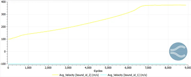
• In the above velocity plot, we easily observe that at the inlet velocity is gradually decreases due to increase in pressure at inlet
• At the outlet, we observe that the velocity is gradually increasing due decrease in pressure.
• At inlet the velocity is decreased and reaches to -100 m/s and at the outlet the velocity is increased and reaches to 360 m/s.
• It occurs since the pressure is inversely proportional to the velocity.

Pressure

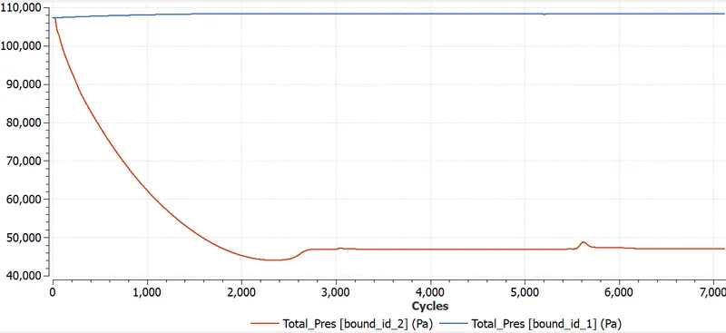
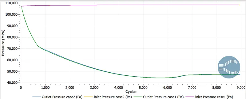
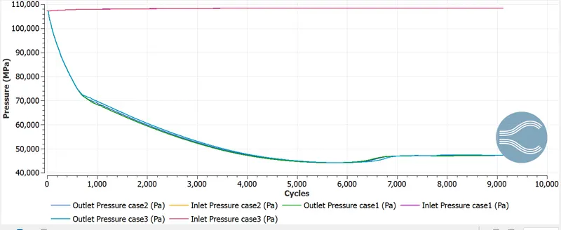
• At the inlet plot of pressure, we observe that initially total and static pressure is same which is 108,310Pa. And we also know that total pressure = static pressure+dynamic pressure and initially dynamic pressure is zero.
• As the cycles going on the static pressure is going to decrease due to increase in dynamic pressure.
• After 1000 cycles the static pressure is going to decrease rapidly due to fastly movement of fluid.

Mach No.

`M=u/c`

Where u is the local flow velocity and c is the speed of sound.

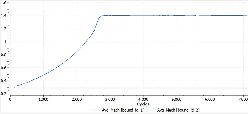
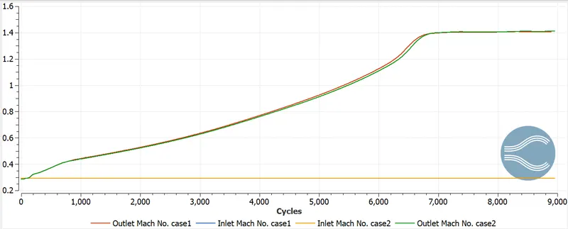
In this case we are taken, the velocity along the x-axis is 100 m/s and roughly the speed of sound is taken 340. So the inlet mach no is 0.289 approximately.

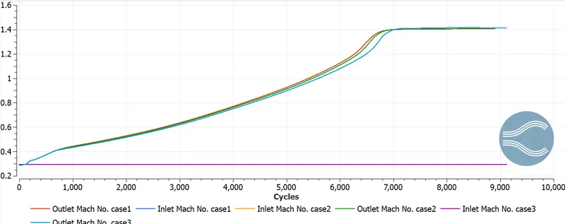
In the avove graph we observe that at the inlet mach no is 2 and there ia an increase in mach no at outlet. Across the expansion fan the flow accelerates and then Mach number increases. At the outlet the value of mach number is 1.4. As there is shock occuring that's why increase in velocity and also increase in Mach number happening.

Temperature

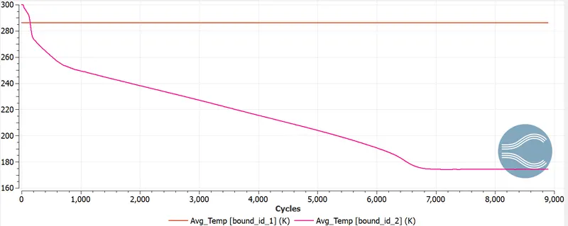
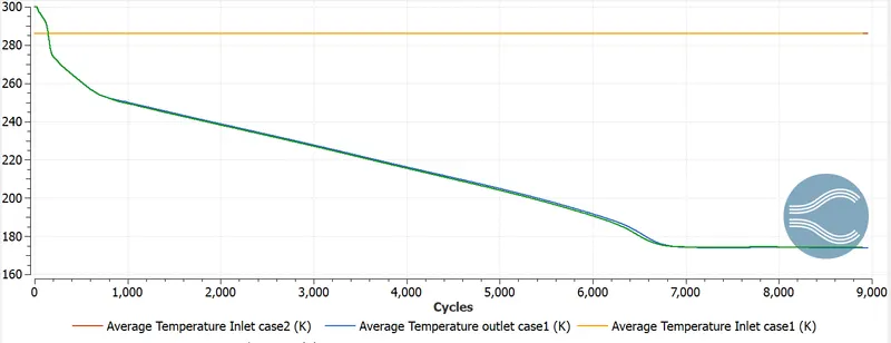
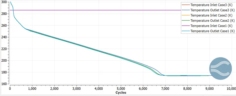
Inlet temperature is assigned as 286K. Outlet static temperature starts to decrease due to expansion and settles at 175K.

Total Cells

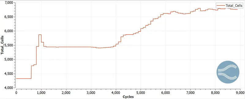
Above graph represent the total no of cells which is approximately 6,700. The above setting that the adaptive mesh refinement is start after 5,800 and that's why there is an sudden increase occur in the no of cells. Because after 5,800 iterations mesh is going to refine and also the capturing of shock wave are also started here.

Contours

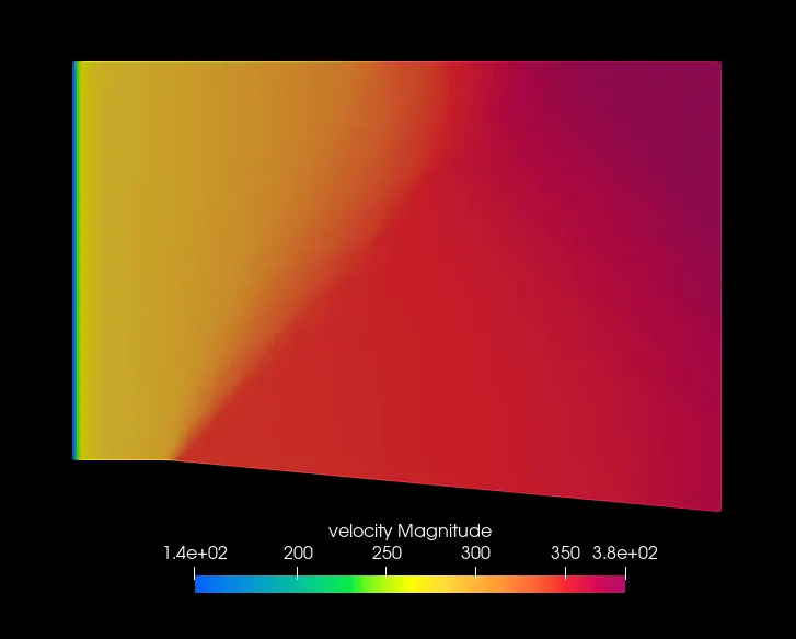
Velocity-Pressure-Temperature

------------------------------------------------------------------------------------------------------------------------

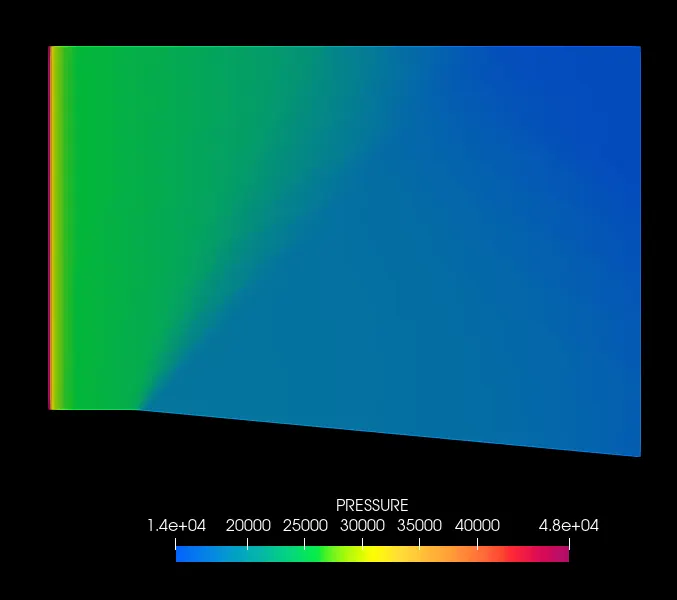
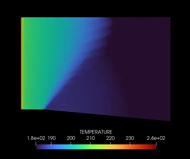
Subsonic case 2: SGS criterion 0.025.

Mesh

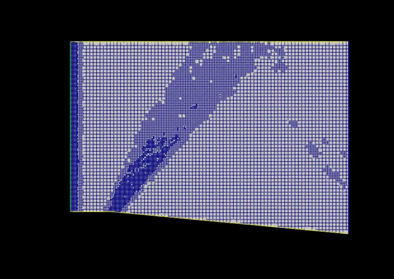
Plots

Mass Flow Rate

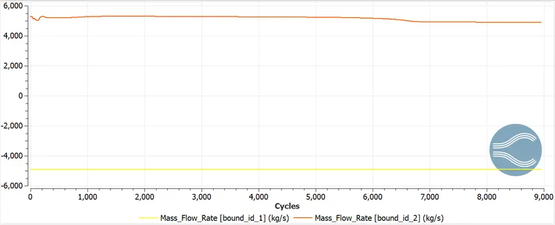
It can be observed that equation of continouity holds and mass flow rate from inlet to outlet is converging.

Average Velocity

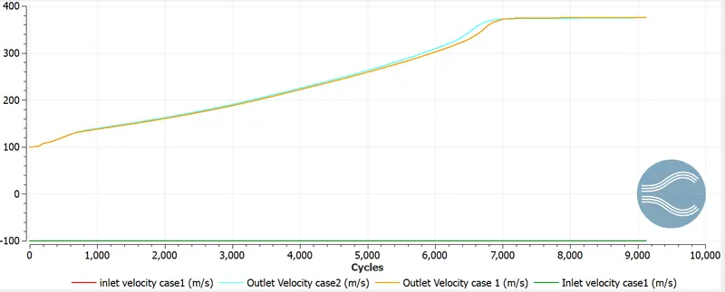
At inlet the velocity is decreased and reaches to -100 m/s and at the outlet the velocity is increased and reaches to 360 m/s. It can be observed that for SGS case 2 (0.025) is converged faster that case 1. This is due to more refined mesh.

Pressure

Mach No.

Temperature

Total Cells

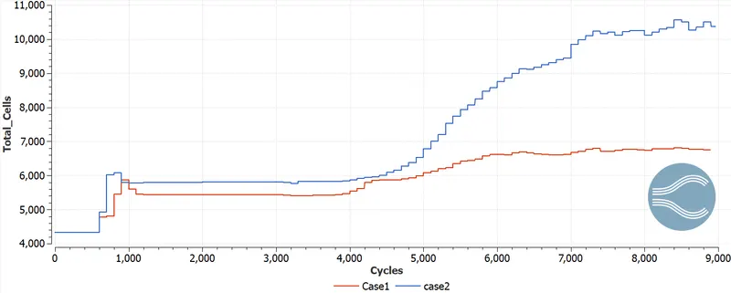
Total Cell count reached 10370 in case 2.

Contours

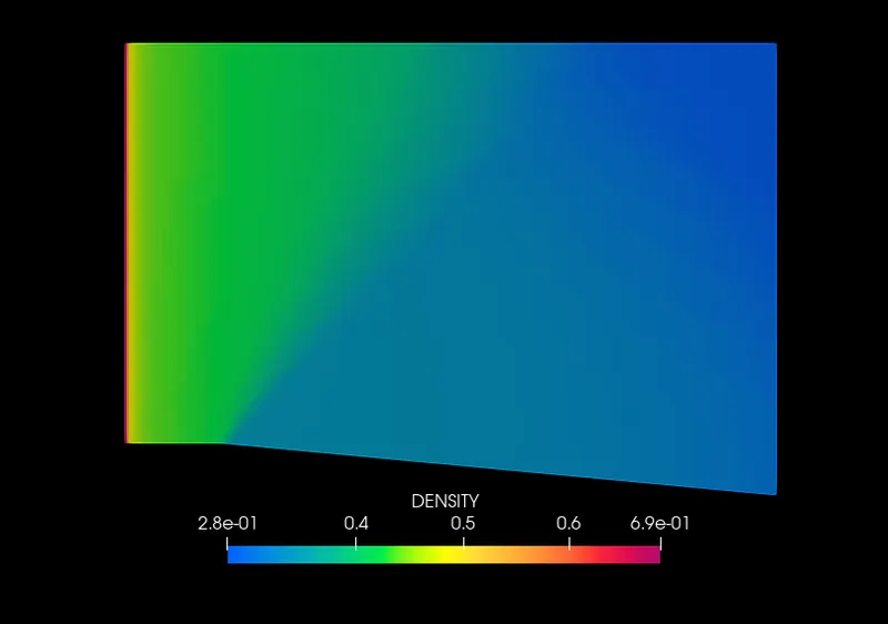
Pressure-Velocity-Temperature-Density

---------------------------------------------------------------------------------------------------------------

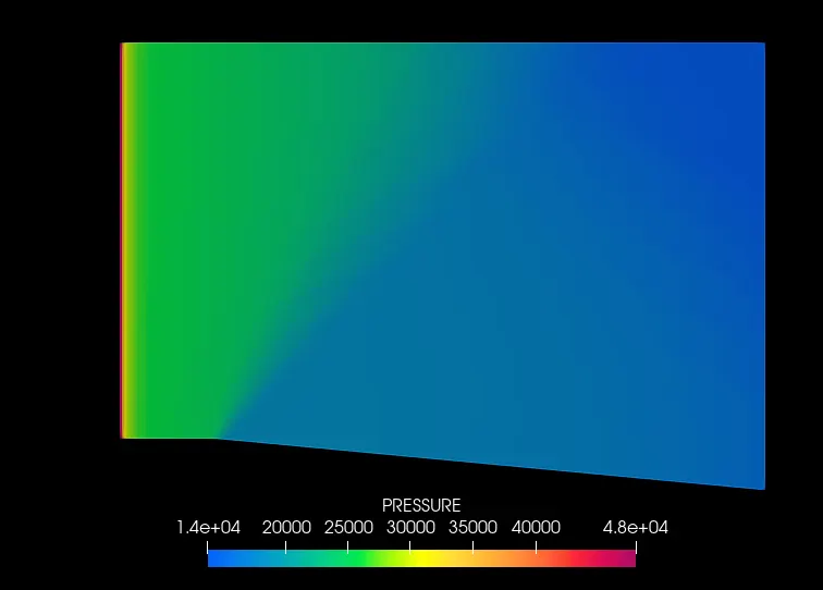
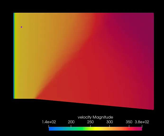
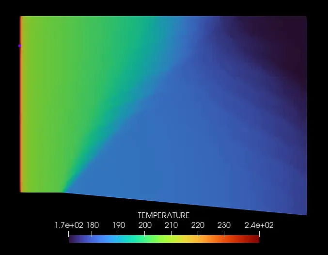
Subsonic case 3: SGS criterion 0.01.

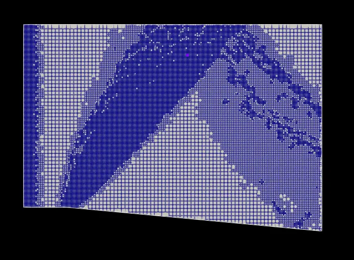
Mesh

Plots

Mass Flow Rate

It can be observed that equation of continouity holds and mass flow rate from inlet to outlet is converging.

Average Velocity

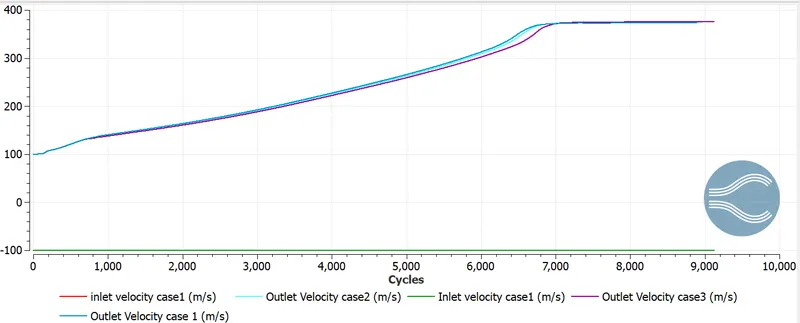
At inlet the velocity is decreased and reaches to -100 m/s and at the outlet the velocity is increased and reaches to 360 m/s. It can be observed that for SGS case 3 (0.01) is converged faster that case 2. This is due to more refined mesh.

Pressure

Mach No.

Temperature

Total Cells

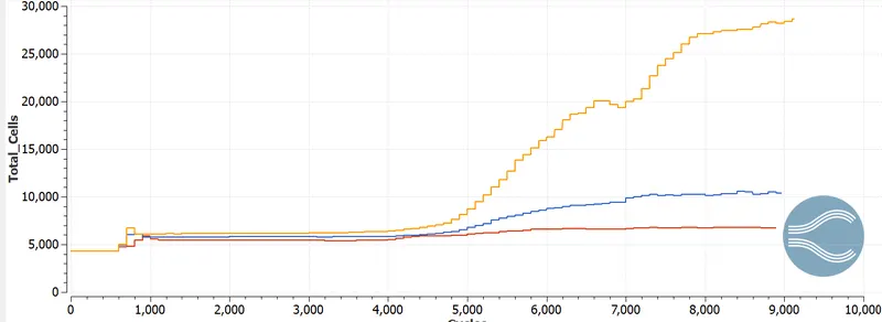
Total cell count reached 28314 in case 3.

Contours

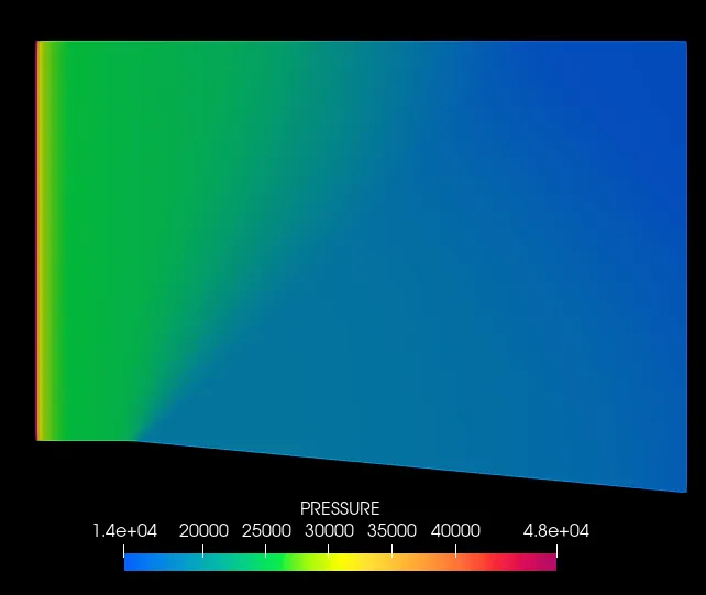
Pressure-Velocity-Temperature-Density

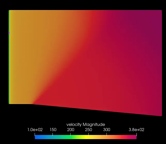
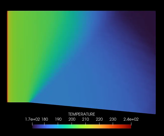
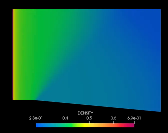
Animation

Velocity

Pressure

----------------------------------------------------------------------------------------------------------------

SUPERSONIC SIMULATION

CASE 1

Boundary Conditions

Inlet -

• The boundary type is INFLOW
• Pressure Boundary Conditions- Zero Normal Gradient (Neumann Boundary)
• Velocity Boundary Conditions-100 m /sec and the velocity of sound is 340 m/sec

Mach number =Velocity of the object / velocity of the sound =100/ 340 = 0.294

• The temperature should be 286.1k and
• Add species 02=0.23 N2=0.77

Outlet

• The boundary type is OUTFLOW
• Pressure Boundary Conditions- Zero Normal Gradient (Neumann Boundary)
• Velocity Boundary Conditions- Zero Normal Gradient (Neumann Boundary)
• The temperature should be 300 k and
• Add species 02=0.23 N2=0.77

Front, Back, Top and Bottom Boundary Conditions:

• For the Front wall boundary should be the 2D wall type.
• For the Back wall Boundary type should be the 2D wall type.
• For the Top and Bottom wall the boundary type is WALL type with the slip condition as a boundary condition and temperature should be 300K.

Boundary Conditions

Inlet -

• The boundary type is INFLOW
• Pressure Boundary Conditions- Zero Normal Gradient (Neumann Boundary)
• Velocity Boundary Conditions-100 m /sec and the velocity of sound is 340 m/sec

Mach number =Velocity of the object / velocity of the sound =100/ 340 = 0.294

• The temperature should be 286.1k and
• Add species 02=0.23 N2=0.77

Outlet

• The boundary type is OUTFLOW
• Pressure Boundary Conditions- Zero Normal Gradient (Neumann Boundary)
• Velocity Boundary Conditions- Zero Normal Gradient (Neumann Boundary)
• The temperature should be 300 k and
• Add species 02=0.23 N2=0.77

Front, Back, Top and Bottom Boundary Conditions:

• For the Front wall boundary should be the 2D wall type.
• For the Back wall Boundary type should be the 2D wall type.
• For the Top and Bottom wall the boundary type is WALL type with the slip condition as a boundary condition and temperature should be 300K.

---------------------------------------------------------------------------------------------------------------------------

---------------------------------------------------------------------------------------------------------------------------

Validation of Supersonic Flow :

To validate our results we need to compare analytical and numerical results.We can get the analytical values by doing
following calculation:-

`f=sqrt((gamma+1)/(gamma-1))arctansqrt(((gamma-1)/(gamma+1))*(M^2-1))-arctan(sqrt(M^2-1))`

and

`f(2)=f(1)+theta`

From the John D Anderson text we got value for

`f(2)=26.37deg`

`f(M2)=theta+f(M1)`

We got `M2=2.2`.

For temperature,pressure and density,we will use following formulae ,

`P2=P1*[(1+((gamma-1)/2)*M1^2)/(1+((gamma-1)/2)*M2^2)]^(gamma/(gamma-1))`

`T2=T1*[(1+((gamma-1)/2)*M1^2)/(1+((gamma-1)/2)*M2^2)]`

`rho2=rho1*[(1+((gamma-1)/2)*M1^2)/(1+((gamma-1)/2)*M2^2)]^(1/(gamma-1))`

Given initial conditions :

T= 286 K, `rho=1.23(kg)/(m^3)`, P = 1 bar

And from analytical calculations at outlet we got following results,

`T_2=269.53k`

`P_2=0.729` bar`

`rho_2=1.124 (kg)/(m^3)`

---------------------------------------------------------------------------------------------------------

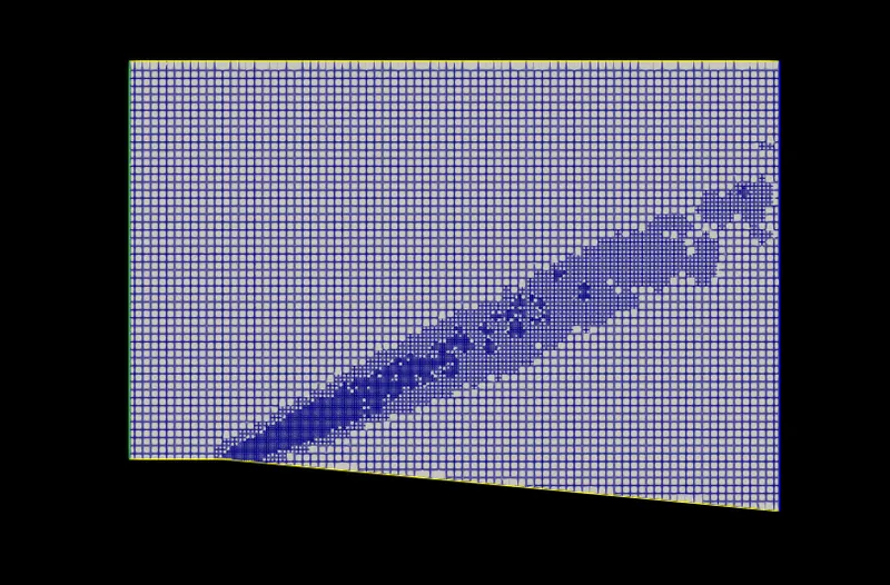
Case 1 SG Criterion=0.05K

Mesh

Plots

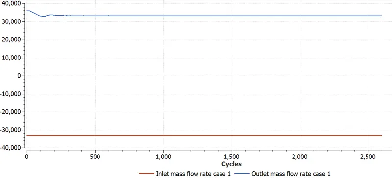
Mass-flow rate

Mass flow rate at inlet and outlet. The Equation of continuity is followed properly.

Pressure

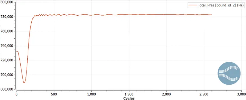
From numerical methods, Pressure value converges with 0.782bar.

Pressure from analytical adiabatic calculations is 0.729.

Error=`(((0.782-0.729)*100)/0.729)=7.27%`

Temperature

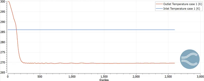
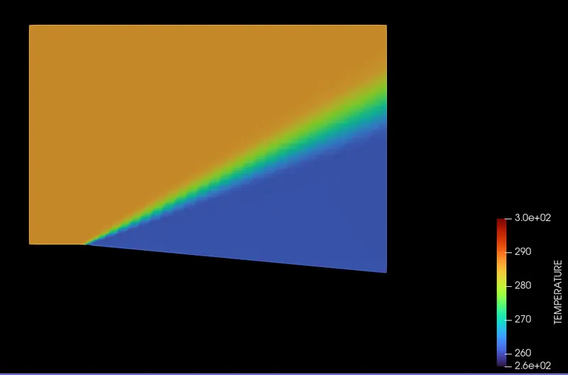
Outlet temperature=269.58K

Analytical Outlet temperature=269.53

Error=`(((269.58-269.53)*100)/269.53)=0.0185%`

Velocity

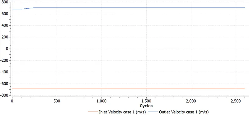
Oultlet Velocity=699.9m/s

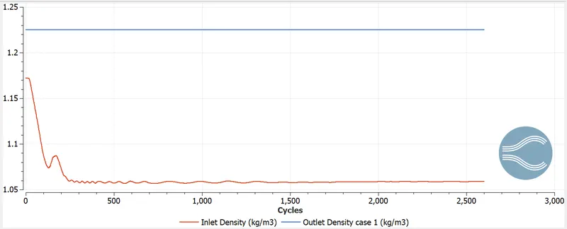
Density

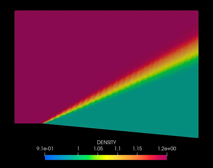
Density at outlet=1.22523

Analytical Density at outlet=1.124

Error=`(((1.22523-1.124)*100)/1.124)=9%`

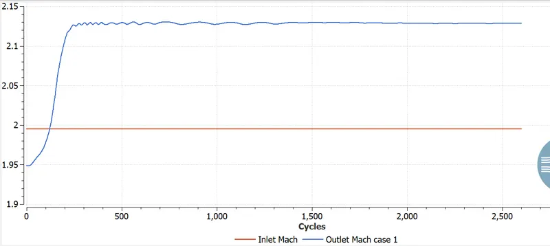
Mach number

Outlet Mach Number=2.12851

Analytical Mach Number at outlet=2.2

Error=`(((2.2-2.12851)*100)/2.2)=3.2495%`

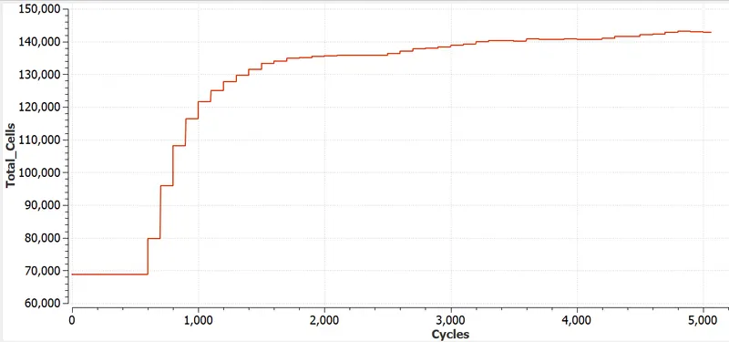
Total Cell

Maximum number of Cells= 7766

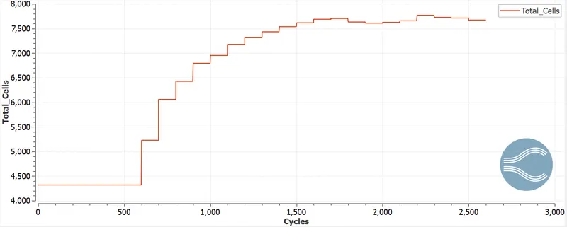
Cellcount, does not remain constant in this case, as the mesh is generated individually for each timestep. We can notice the cell count stays constant for the first ~600 cycles, after 600 cycles adaptive mesh refining is enabled. The cell count also stabilises towards the end when steady state happens. Total Cell count is always roughly 4 times the value for each Core.

------------------------------------------------------------------------------------------------------------

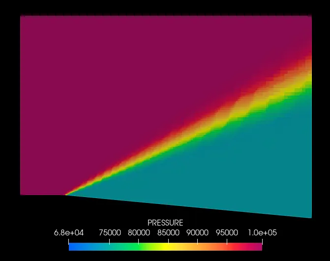
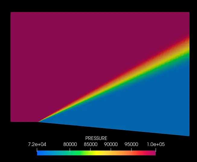
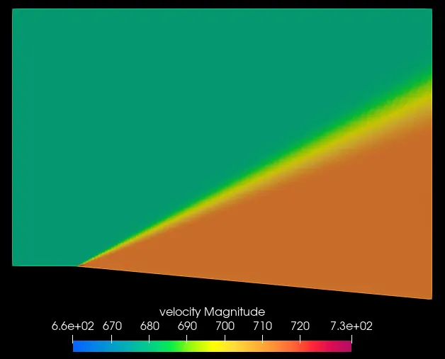
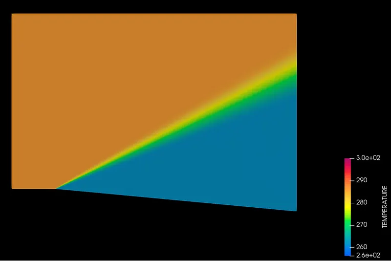
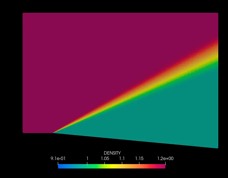
Contours

Pressure-Velocity

Temperature-Density

--------------------------------------------------------------------------------------------------------------

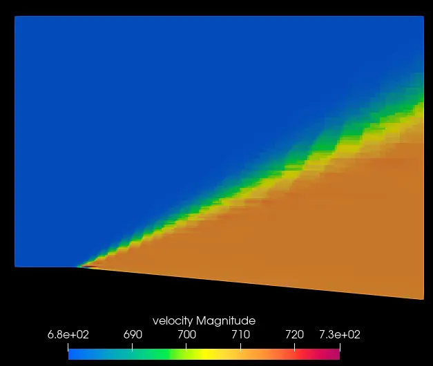
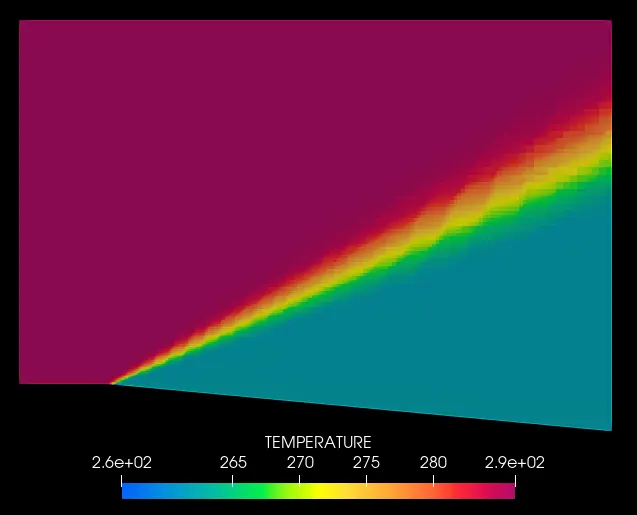
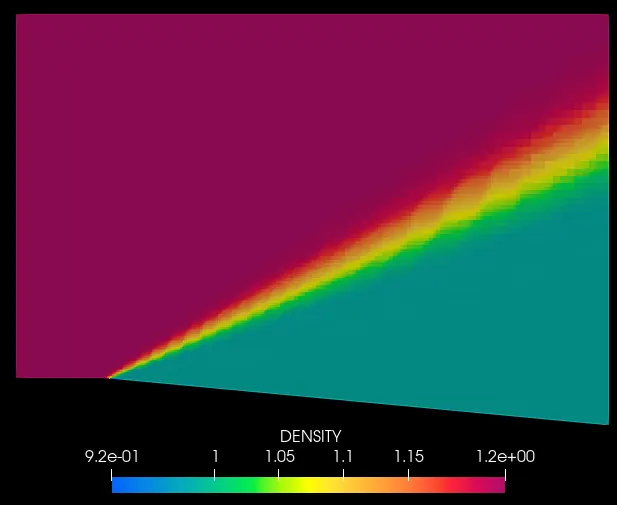
Case 2 SG Criterion=0.025K

Mesh

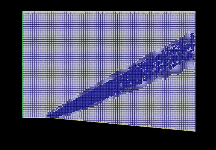
Plots

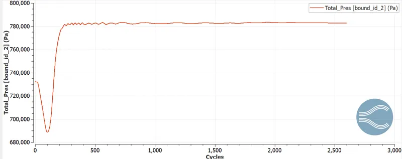
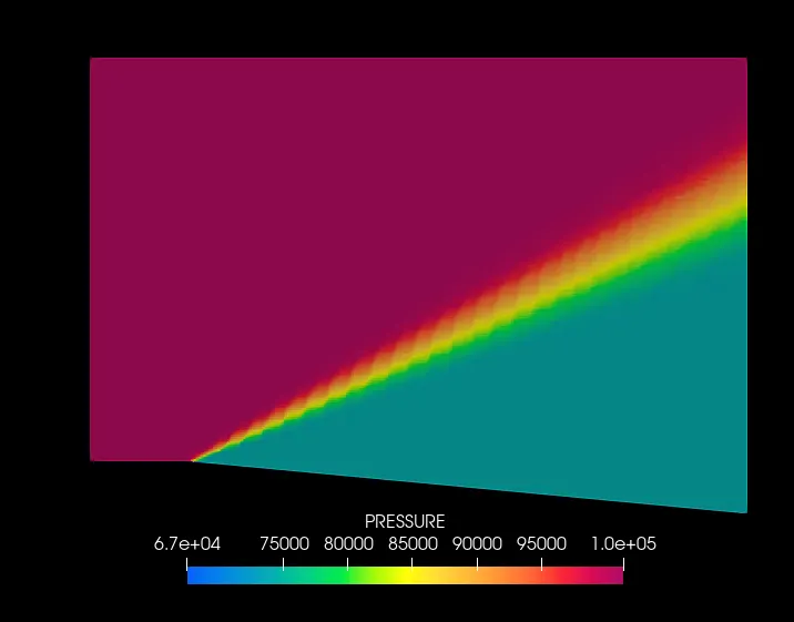
Pressure

From numerical methods, Pressure value converges with 0.782bar.

Pressure from analytical adiabatic calculations is 0.729.

Error=`(((0.782-0.729)*100)/0.729)=7.27%`

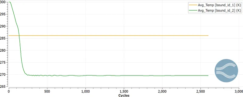
Temperature

Outlet temperature=269.559K

Analytical Outlet temperature=269.53

Error=`(((269.559-269.53)*100)/269.53)=0.0107%`

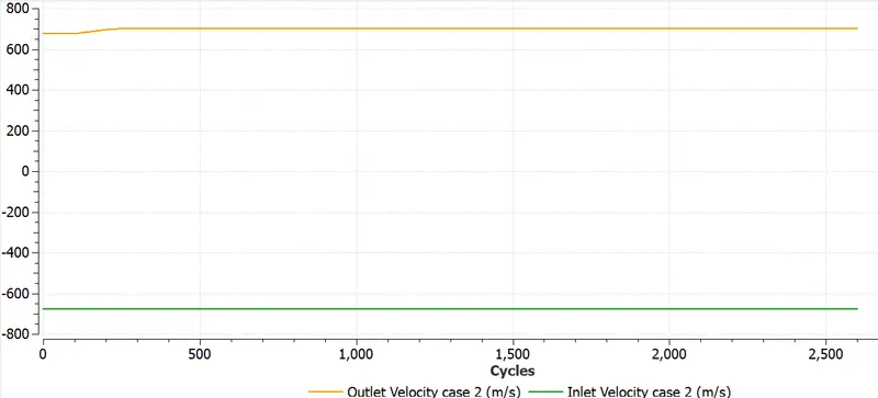
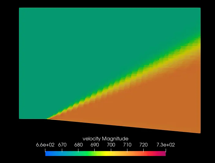
Velocity

Oultlet Velocity=700.192m/s

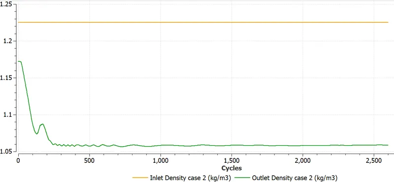
Density

Density at outlet=1.22523

Analytical Density at outlet=1.124

Error=`(((1.22523-1.124)*100)/1.124)=9%`

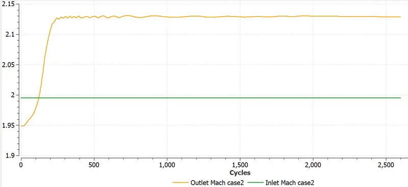
Mach number

Outlet Mach Number=2.12851

Analytical Mach Number at outlet=2.2

Error=`(((2.2-2.12851)*100)/2.2)=3.2495%`

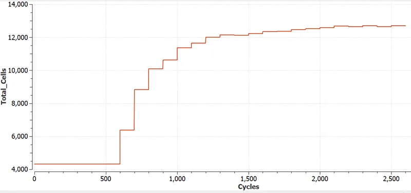
Total Cell Count

Maximum number of Cells= 12706

------------------------------------------------------------------------------------------------------------

Contours

Pressure-Velocity

Temperature-Density

--------------------------------------------------------------------------------------------------------------

Case 3 SG Criterion=0.01K

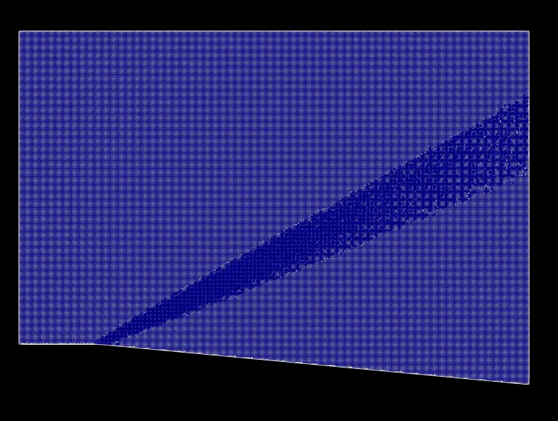
Mesh

Plots

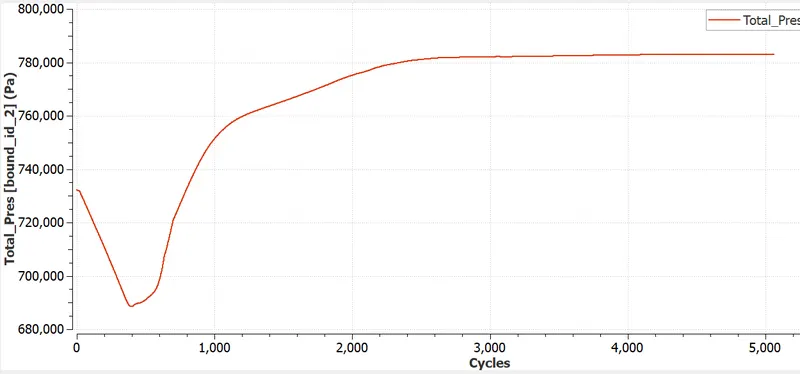
Pressure

From numerical methods, Pressure value converges with 0.782bar.

Pressure from analytical adiabatic calculations is 0.729.

Error=`(((0.782-0.729)*100)/0.729)=7.27%`

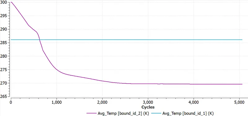
Temperature

Outlet temperature=269.559K

Analytical Outlet temperature=269.53

Error=`(((269.559-269.53)*100)/269.53)=0.0107%`

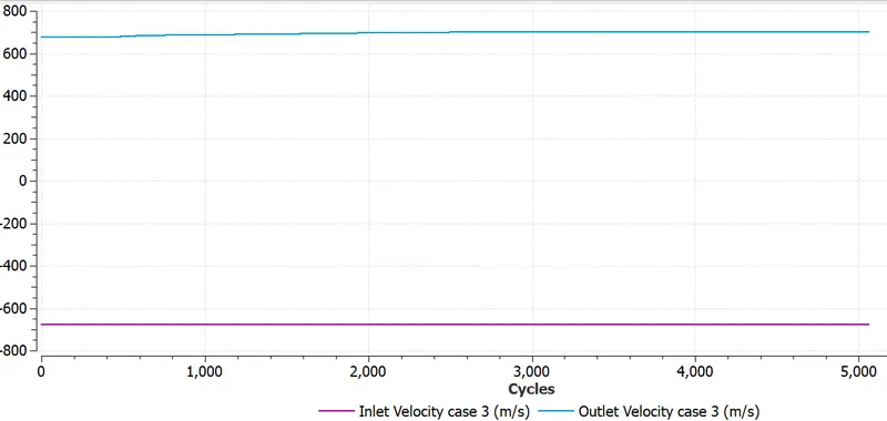
Velocity

Oultlet Velocity=700.192m/s

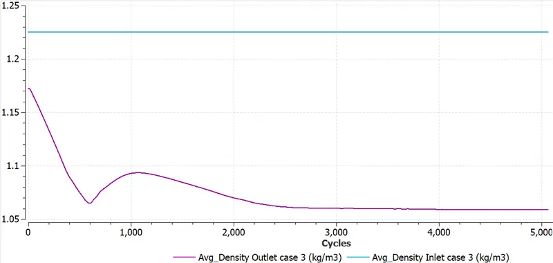
Density

Density at outlet=1.22523

Analytical Density at outlet=1.124

Error=`(((1.22523-1.124)*100)/1.124)=9%`

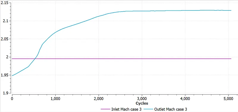
Mach number

Outlet Mach Number=2.12851

Analytical Mach Number at outlet=2.2

Error=`(((2.2-2.12851)*100)/2.2)=3.2495%`

Total Cell Count

Maximum number of Cells= 143159

------------------------------------------------------------------------------------------------------------

Contours

Pressure-Velocity

Temperature-Density

Animation

Mesh

Velocity

Note: We can notice a sharp decrease in the size of the expansion fan when adaptive meshes are generated, this is due to more precision gained when calculating the solution with adaptive mesh refining.

Pressure

---------------------------------------------------------------------------------------------------------------------

CONCLUSION

• We are successfully simulating the supersonic and subsonic prandtl flow in a 2D duct having a sharp corner was setup and run in converge CFD. Various contours plots of velocity, pressure, density and temperature were studied.
• We ran the simulation at different SGS values and concluded the results.
• We also run the simulation using the velocity 680 m/s and 100 m/s.
• Changing the SGS values changes the number of cells that are formed during meshing. As mentioned above when Sub-grid temperature is greater than SGS value, the mesh is refined.
• For the low value of SGS(0.01 and 0.025 more cells are refined than the higher value of SGS(0.5).
• The inlet Mach no where flow enter to the geometry is 2 and the outlet mach no is 2.15 which correspond to an outlet velocity 700m/s as compared to the inlet velocity 680m/s.

Effect of SGS parameter on shock location and total cell count

Cell Count: As the SGS parameter decreases, the total cell count increases. In other words, for small SGS parameter AMR refines the mesh for more number of cells in and around the shock wave.

Shock Location: For high SGS parameter, the mesh refinement area is very small like (SGS = 0.1) and for the small SGS parameter, the mesh refinement area spans from the sharp edge till the outlet boundary.

Subsonic Vs Supersonic flow comparison

In supersonic flow, the prandtl mayer expansion fan is clearly visible and the mesh refinement is also in the shock region. Whereas on the other hand ,in the case of subsonic flow, the prandtl mayer shock fan is not clearly visible and even the mesh refnement is not visible. This is because there are no sudden fluctuations in pressure, velocity, temperature or density or in other words shock.

Also the average Mach number inceases from the inlet to the outlet in case of supersonic flow and deceases in case of subsonic flow.