Week 5: Prandtl Meyer Shock problem

Week 5: Prandtl Meyer Shock problem

Aim:

• To do a literature search on what BC's are typically used for shock flow problems.
• To understand the reason behind the usage of Neumann Boundary condition at outlet for supersonic flow.
• To explain what a shock waves are and the physics behind it.
• To explain about the effect of SGS parameter on shock location.
• To show the mesh generation using PARAVIEW.

Theory and Introductions:

Prandtl Meyer Shock Problem:

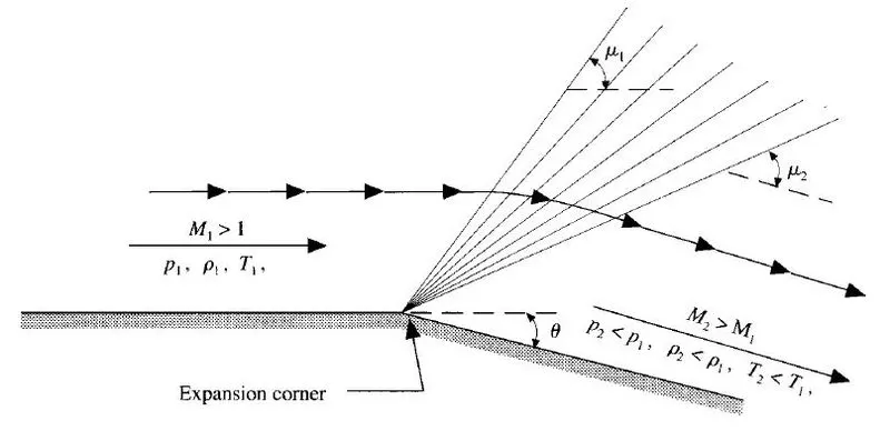
• Prandtl Meyer expansion fan is a two dimensional simple wave, which occurs when a supersonic flow turns around a convex corner.
• The fan consists of infinite number of Mach waves, diverging from a sharp corner. When a flow turns around a smooth and circular corner, these waves can be extended backwards to meet at a point.
• Across the expansion fan, the flow accelerates and the Mach number increases, while the static pressure, temperature and density decrease. Since the process is isentropic the stagnation properties remain constant across the fan.

Literature search on Boundary Conditions used for shock flow problems:

For solving the steady state flow appropriate boundary conditions are needed. It is one of the required components of the mathematical model. On the other hand for solving transient flow, appropriate initial conditions are also required.

The choice of the boundary condition is very important because a wrong selection of the boundary condition may lead to divergence or even lead to convergence of incorrect solution.

Types of Boundary Conditions:

• Dirichlet Boundary Condition.
• Neumann Boundary Condition.
• Robin Boundary Condition.
• Mixed Boundary Condition.
• Cauchy Boundary Condition.

Dirichlet Boundary Condition:

The Dirichlet boundary condition is imposed on an ordinary or a partial differential equation, it specifies the values that a solution needs to take along the boundary of the domain.

In Finite Element Method, essential or Dirichlet boundary condition is defined by weighted-integral form of a differential equation. The dependent unknown u in the same form as the weight function w appearing in the boundary expression is termed a primary variable, and its specification constitutes the essential or Dirichlet boundary condition. In fluid dynamics the no-slip condition for viscous fluid states that at a solid boundary, the fluid will have zero velocity relative to the boundary.

Neumann Boundary Condition:

The Neumann Boundary Condition is a condition named after Carl Neumann. When imposed on an ordinary or a partial differential equation, the condition specifies the values of the derivative applied at the boundary of the domain.

It is possible to describe the problem using other boundary conditions: a Dirichlet boundary condition specifies the values of the solution itself (as opposed to its derivative) on the boundary, whereas the Cauchy boundary condition, mixed boundary condition and Robin boundary condition are all different types of combinations of the Neumann and Dirichlet boundary conditions.

Robin Boundary Condition:

The Robin boundary condition consists of a linear combination of the values of the field and its derivatives on the boundary. Thus, it can also be said to be the linear combination of the Dirichlet and Neumann boundary conditions.

Mixed Boundary Condition:

It consists of applying different types of boundary conditions in different parts of the domain. The mixed boundary condition differs from the Robin condition because the latter consists of different types of boundary conditions applied to the same region of the boundary, while the mixed condition implies different types of boundary conditions applied to different parts of the boundary.

Cauchy Boundary Condition:

The Cauchy boundary condition is a condition on both the unknown field and its derivatives it differs from the Robin condition because the Cauchy condition implies the imposition of two constraints (1 Dirichlet + 1 Neumann), while the Robin condition implies only one constraint on the linear combination of the unknown function and its derivatives.

Shock flow boundary condition at outlet:

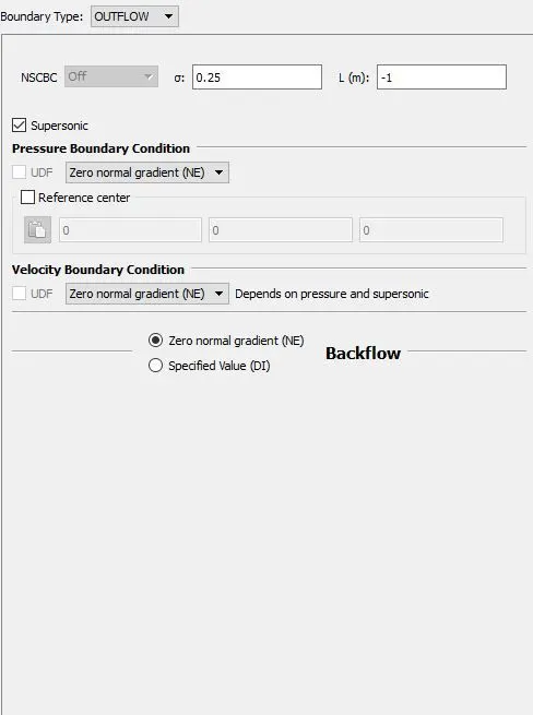
The values of the variables like temperature, Mach no, velocity, pressure are not available at the initiation of the problem. At a supersonic outlet boundary condition, nothing is specified and all listed variables are extrapolated from the interior domain. Only the Normal derivative (Normal with respect to the outlet boundary) of variables are specified as 0 (or Zero Gradient). However, if any pressure value or velocity is specified at the outlet the solution will not converge and become unstable. In the Neumann boundary condition, the value of the gradient of the dependent variable is provided along the boundary of the domain. In supersonic flow, characterized by abrupt changes in state parameters, a steady value of parameters. Hence extrapolated Neumann boundary conditions are employed for shock waves and supersonic conditions.

Shock wave and the physics behind it:

At a molecular level, fluid particles travels in a continuum. When an obstruction is suddenly introduced into the flow, the particles in front of it slow down instantaneously creating an increase in local pressure. Since the fluid is a continuum, the information of whatever happens in one place is transmitted to the other regions in the form of pressure waves. This pressure waves then causes the oncoming fluid to adjust its properties. The sound also travel in the form of compressions and rarefactions through a medium. The information Propagation in a fluid happens through acoustic waves which travel at the speed of sound. If the particles are travelling faster than the speed of sound, the information transfer cannot happen faster than the speed of sound, these fast moving particles don't have any information about the obstruction in front until they reach it. The moment they reach it, an extreme collision of particles with themselves and the object which manifest itself as a shockwave.

Mach number is a dimensionless number which is very important while studying shocks.

Mach (M) = Velocity of the fluid / Speed of sound in medium.

So, if the Mach number is greater than 1, it means the fluid travels faster than the speed of sound and there's no time for information to propagate. These are called as supersonic flows.

A moving shock is called as a shockwave which is very thin and in this region, the fluid undergoes sudden changes in properties. When a stationary objects emits sound waves at a certain frequency, the waves are generally spherical in nature and travel at the speed of sound. The moment an object compress, increasing the apparent frequency this effect is called as Doppler Effect. When the object travels faster than the speed of sound, the sound waves that are emitted from a cone known as Mach Cone.

Geometry setup:

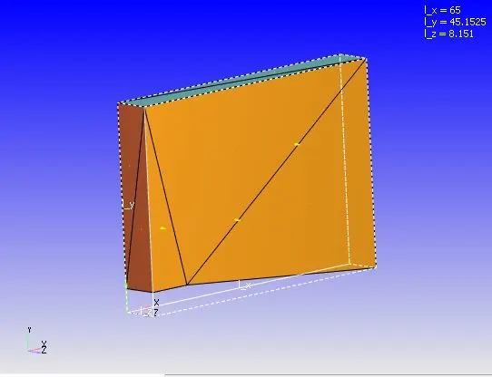
• As the geometry was provided in STL format it is imported in the CONVERGE studio software by using the file--> import --> import STL command.

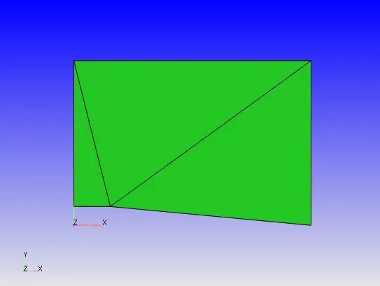
• Diagnosis toolbar is used for geometry check-up.
• Converge assumes the dimensions in meters. So we are scaling down the geometry with the factor of 0.001. By using the following command Geometry --> Transform --> Scale --> Entity Type --> Entire Surface --> Scale Factor --> Uniform= 0.001 --> Apply.

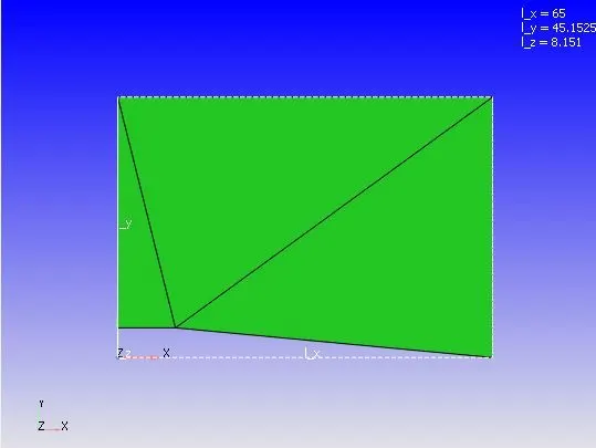
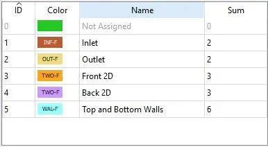
• In the next step the boundaries are flagged with names.

Case Setup:

• The application type is fixed with time based.
• Then click on Materials which is present in the right side of the window that is case setup tree and select the Predefined mixtures as Air.
• Click on the Gas simulation and Global Transport parameter and retain the same values.
• Click on Species and then add O2 and N2.
• Click on Run Parameters and under the solver tab choose the solver as Steady-State Solver. Set the simulation mode to Full Hydrodynamic and the gas flow solver as compressible.
• Then under "Misc" tab check the Steady-state monitor and uncheck the use shared memory boxes.
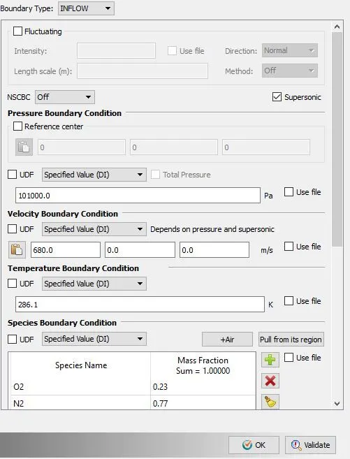
• Then coming to Boundary Conditions click on Boundary--> Inlet -->Specify the inlet pressure value as 101000.0 Pa and select the predefined mixture as Air which contains N2 of 77% and O2 of 23% and then under the Velocity Boundary Condition choose the specified value and enter the velocity value in X axis as 680 m/s which is supersonic (Mach 2) and under the Temperature boundary condition choose specified value and allocate the temperature value with 286.1K Considering this as Dirichlet Boundary Condition.

• Then in Outlet--> Specify the boundary type as Outflow and make this outlet as Neumann Boundary Condition.

• Then assign the Front 2D and Back 2D as TWO_D.
• The Top and Bottom walls are assigned Wall with Slip boundary condition.
• Then under the Simulation Parameter --> Run Parameters select the Steady-state monitor --> add config and then click on add option to add the variables to be monitored.
• The Monitor start display is a parameter that ensures that the simulation runs for a certain number of cycles before the variable can be monitored. This is especially useful in transient simulations when we want the solution to run for a particular amount of time before checking the convergence, if the steady state results are also required.
• Sample size denotes the number of cycles or seconds over which the variable is checked to see if the solutions have converged.
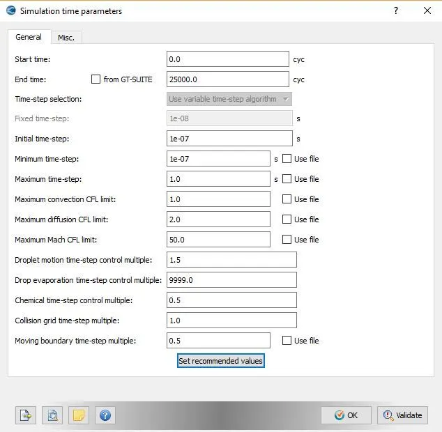
• Then under the Simulation Time Parameters assign the End time and look after the Maximum Convection CFL limit and assign with 1.

• Then click on Solver Parameters [Steady-state] --> Equations --> Pressure --> Make sure that the Preconditioner is set to None. Then under the Steady-state solver control assign the maximum convection CFL limit (final stage) to less than 1 --> Click on Validate --> Click on OK.
• Then under the Initial conditions and Events --> Regions and Initialization --> add a region and rename it as Volumetric Region User Defined by using the F2 option

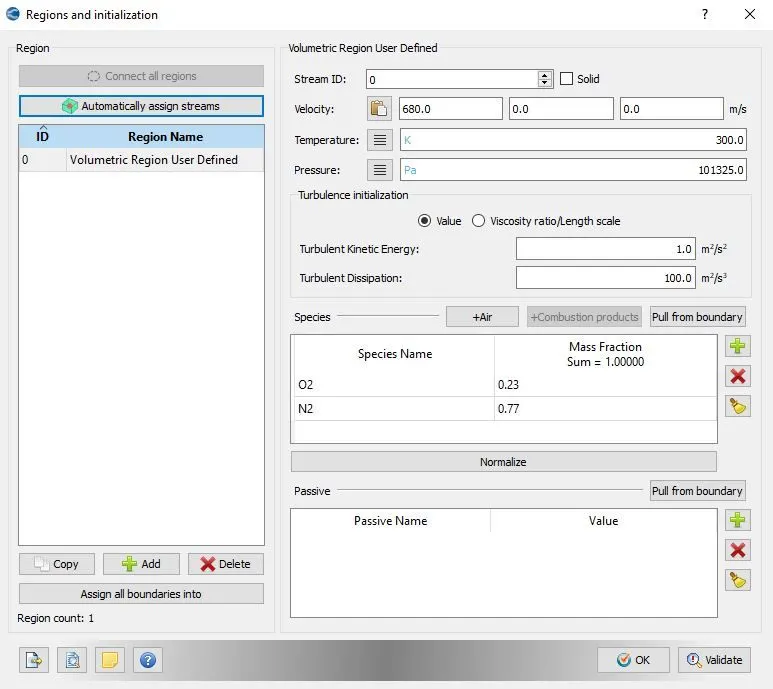
• Then under the boundary conditions assign the region names to the named boundary regions.
• Then under the physical models check the turbulence modelling and set with Reynolds Averaged Navier-Stokes (RANS) and set the turbulence model with RNG K-epsilon.
• Then in the Grid Control parameter --> Base Grid --> Enter the size of the grid.

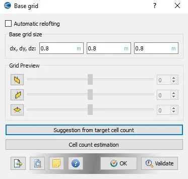
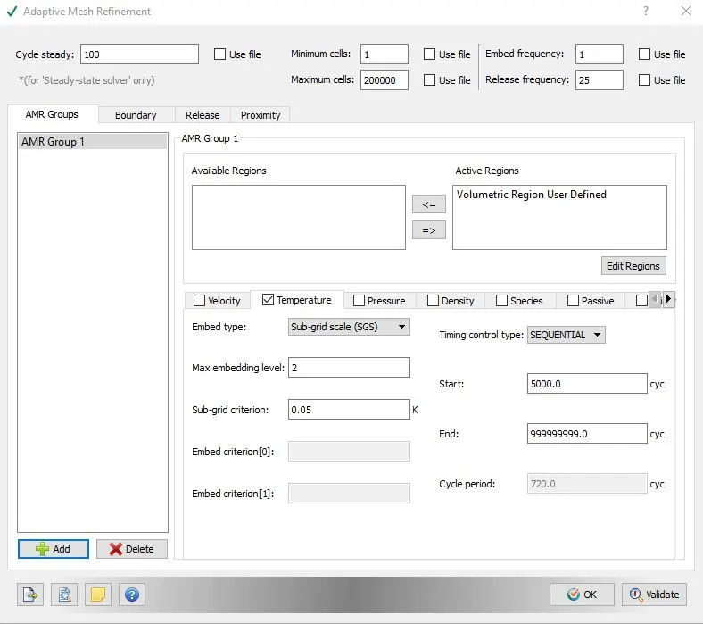
• Then in the Grid control parameter check the "Adaptive Mesh Refinement" option. Adaptive mesh refinement is a method of adapting the accuracy of a solution within certain sensitive or turbulent regions of simulation, dynamically and during the time the solution is being calculated. When the solutions are calculated numerically, they are often pre-determined quantified grids as in the Cartesian plane which constitutes the computational grid or mesh.

The available region is Volumetric Region User Defined which is converted to active regions.

Minimum cells - 1

Maximum cells - 200000

Embedded Type - Sub Grid Scale (SGS)

Temperature scheme is used for AMR with Embed type- SGS

Sub grid criterion - 0.05 K and the value is changed after each simulation to find the difference.

Max embedding level as 2

Timing control type - Sequential

• Then under Output/Post-Processing --> Post Variable Selection --> Add the Mass fraction with O2 and N2
• Then under the Output files --> Writing time intervals --> set the time interval for writing 3D output data files and time interval for writing restarting output.
• Then use CYGWIN to execute the CFD solver.
• Then with the help of Converge CFD the post converting the output files to paraview format is done.
• Paraview is used for Post processing the results.

Results:

Case 1:

Sub-grid criterion = 0.05 K

Mesh:

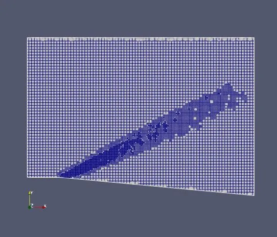
From the mesh profile, the advantage of adaptive mesh refinement parameter is visible. It has embedded the mesh size by 2 levels with the SGS of 0.05 K. This refinement helps in capturing characteristics of the flow through the domain specifically at the sharp corner, to have a better analysis of the shock wave. The mesh refinement with SGS of 0.05 K, it fails to refine the complete expansion fan region, which will affect the analysis of the flow properties in those undefined regions.

Velocity Contour:

Pressure Contour:

Temperature Contour:

Mass flow rate plot:

Velocity plot:

Temperature plot:

Mach plot:

Total cells plot:

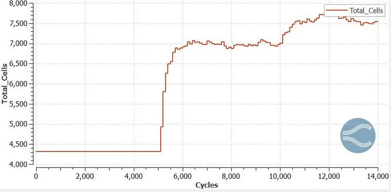
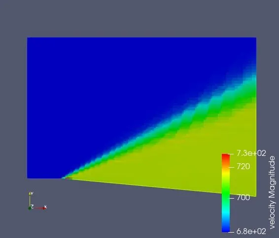
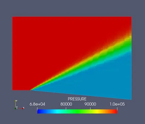
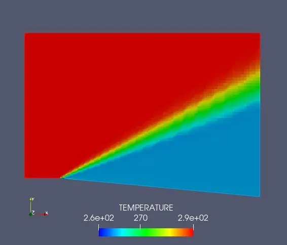
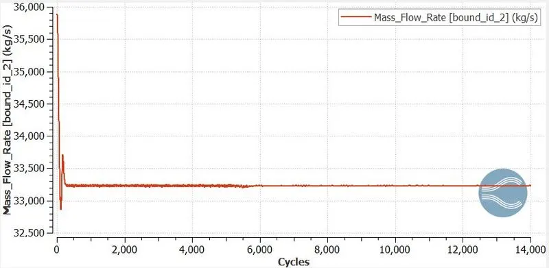
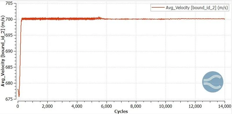
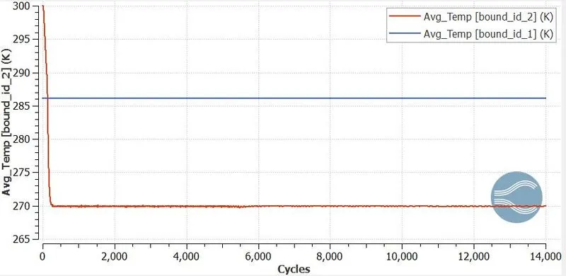
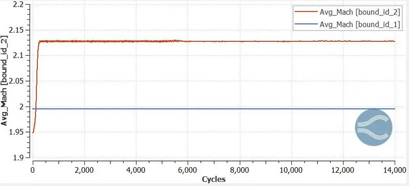
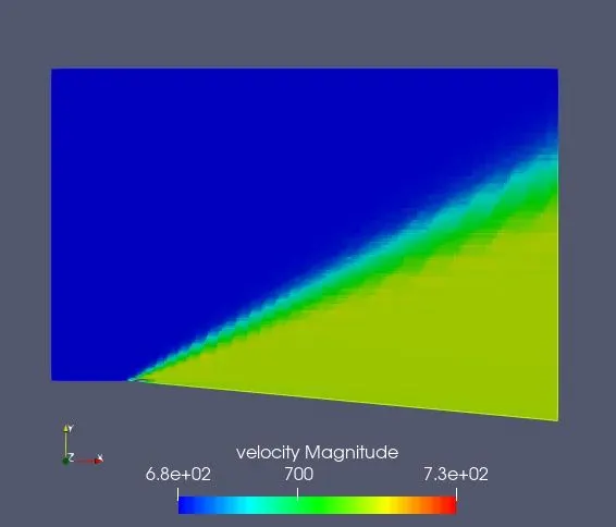
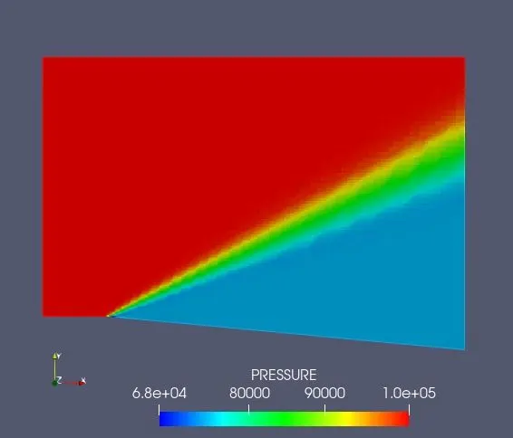
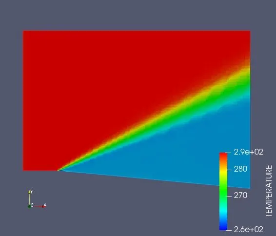
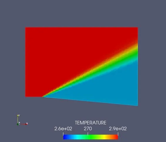
Above plots and contours representing the variation of pressure, velocity, temperature, density and Mach number through the domain length. As the flow propagates through the domain at a speed higher than the speed of sound and with an abrupt increase of domain area, centred expansion waves or centred expansion fan is generated. Hence, with the generation of the Prandtl-Meyer expansion fan, the Mach number and velocity increases whereas the flow properties such as the density, temperature and pressure decreases.

Case 2:

Sub-grid criterion = 0.04 K

Mesh:

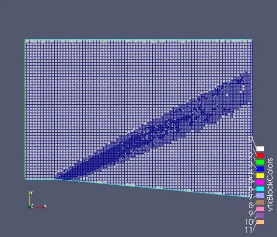
From the mesh profile, the advantage of adaptive mesh refinement parameter is visible. It has embedded the mesh size by 2 levels with the SGS of 0.04 K. This refinement helps in capturing characteristics of the flow through the domain specifically at the sharp corner, to have a better analysis of the shock wave. When compared to the mesh refinement with SGS of 0.05 K, it refines the expansion fan region better, for the analysis of the flow properties in those undefined regions.

Velocity Contour:

Pressure Contour:

Temperature Contour:

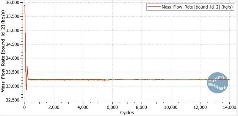
Mass flow rate plot:

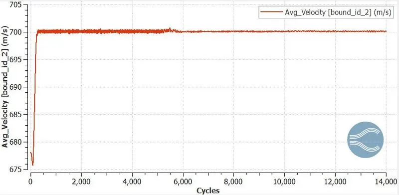
Velocity plot:

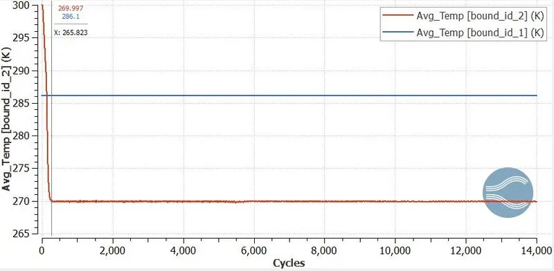
Temperature plot:

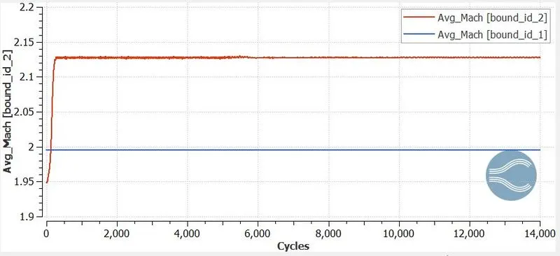
Mach plot:

Total cell plot:

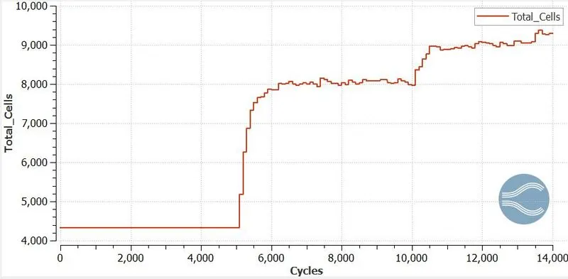
Above plots and contours representing the variation of pressure, velocity, temperature, density and Mach number through the domain length. As the flow propagates through the domain at a speed higher than the speed of sound and with an abrupt increase of domain area, centred expansion waves or centered expansion fan is generated. Hence, with the generation of the Prandtl-Meyer expansion fan, the Mach number and velocity increases whereas the flow properties such as the density, temperature and pressure decreases.

Case 3:

Sub-grid criterion = 0.03 K

Mesh:

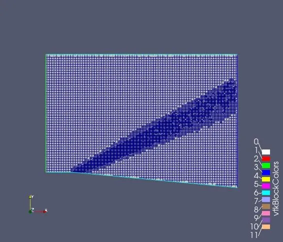
From the mesh profile, the advantage of adaptive mesh refinement parameter is visible. It has embedded the mesh size by 2 levels with the SGS of 0.03 K. This refinement helps in capturing characteristics of the flow through the domain specifically at the sharp corner, to have a better analysis of the shock wave. When compared to the mesh refinement with SGS of 0.03 K, it refines the expansion fan region better, for the analysis of the flow properties in those undefined regions.

Velocity Contour:

Pressure Contour:

Temperature Contour:

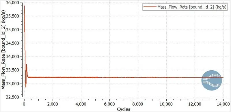
Mass flow rate plot:

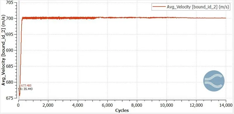
Velocity plot:

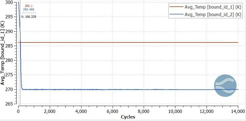
Temperature plot:

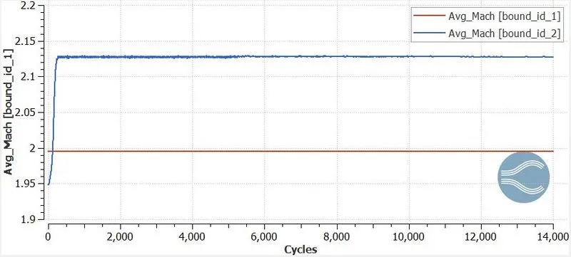
Mach plot:

Total cells plot:

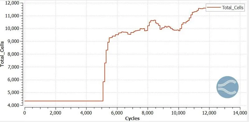
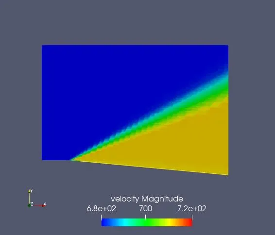
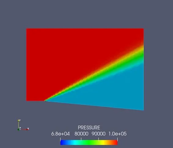
Above plots and contours representing the variation of pressure, velocity, temperature, density and Mach number through the domain length. As the flow propagates through the domain at a speed higher than the speed of sound and with an abrupt increase of domain area, centred expansion waves or centred expansion fan is generated. Hence, with the generation of the Prandtl-Meyer expansion fan, the Mach number and velocity increases whereas the flow properties such as the density, temperature and pressure decreases.

Case 4:

Sub-grid criterion = 0.01 K

Mesh:

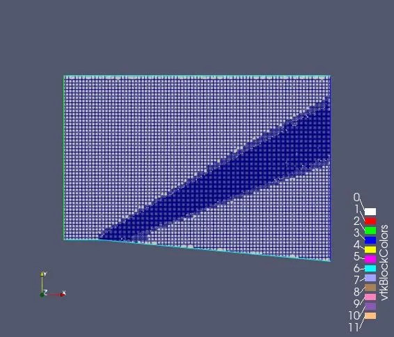
From the mesh profile, the advantage of adaptive mesh refinement parameter is visible. It has embedded the mesh size by 2 levels with the SGS of 0.01 K. This refinement helps in capturing characteristics of the flow through the domain specifically at the sharp corner, to have a better analysis of the shock wave. When compared to the mesh refinement with SGS of 0.03 K, it refines the expansion fan region better, for the analysis of the flow properties in those undefined regions.

Velocity Contour:

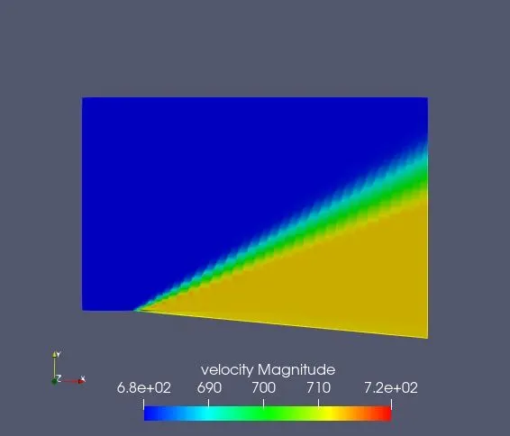
Pressure Contour:

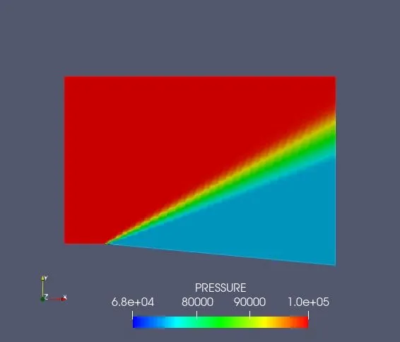
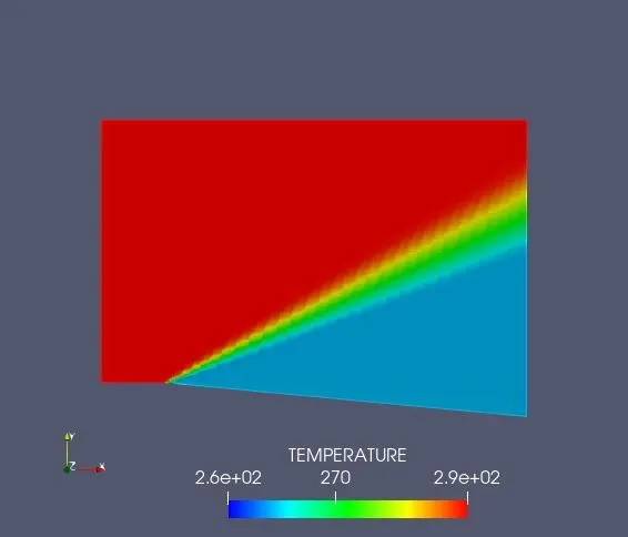
Temperature Contour:

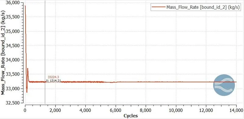
Mass flow rate plot:

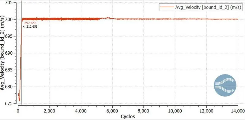
Velocity plot:

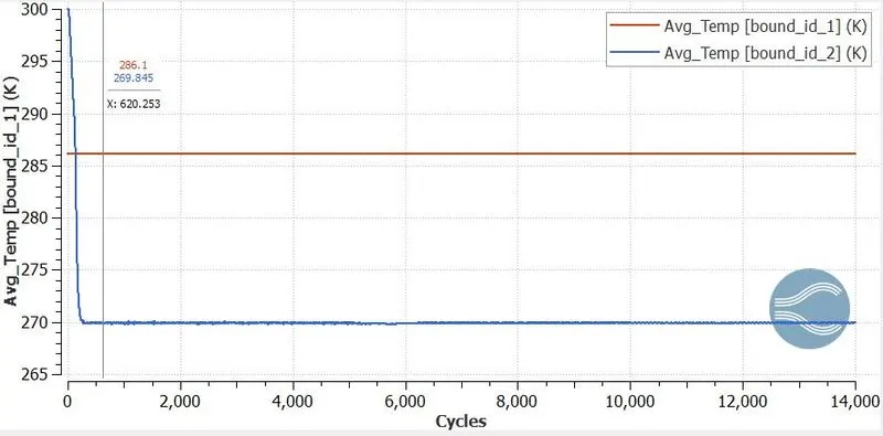
Temperature plot:

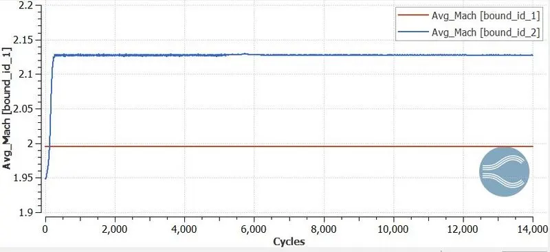
Mach plot:

Total cells plot:

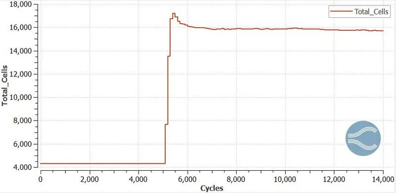
Above plots and contours representing the variation of pressure, velocity, temperature, density and Mach number through the domain length. As the flow propagates through the domain at a speed higher than the speed of sound and with an abrupt increase of domain area, centred expansion waves or centred expansion fan is generated. Hence, with the generation of the Prandtl-Meyer expansion fan, the Mach number and velocity increases whereas the flow properties such as the density, temperature and pressure decreases.

We can predict that the more refined solution and better looking contour towards the end of the fan and along its edges, it has happened due to the lower SGS criterion. From this we could understand that if the SGS criterion value is lower we could get a more refined solution with an increase in mesh sizes and better results.

From the Mach number plot, we can see that the moment it meets the convex corner, expansion fan formed, Mach number is increased, but then towards outlet it normalizes. Since shock flow is an irreversible process, it will cause increase in entropy.

Velocity Animations:

Case 1: https://youtu.be/50_qEASrZC4

Case 2: https://youtu.be/rrn4Di5zeuA

Case 3: https://youtu.be/tpzeJzFdeY4

case 4: https://youtu.be/ILxAq9dBahU

Effect of SGS parameter on shock location and cell count:

1. SGS is sub-grid, which is a mesh refiner in the adaptive mesh refinement that depending on the gradients among the parameters. SGS refines the mesh grid by the variations in the curve of the parameters. This helps in capturing the details in the gradient region. Here gradient refers to the second order PDE. If we specify the value like temperature to be 0.01 degree in the sub grid criterion, then if the rise in temperature in the region above the average temperature of the region the mesh gets finer depending on the scale is set. This adaptive technique provides detailed insight into the turbulent region.

As the value of the SGS parameter decreases, the total cell count increases. For small SGS parameters, AMR refines the mesh for more number of cells in and around the shock waves. As SGS value is lowered it can be observed that refinement of mesh i.e. adaptive mesh refinement at Mach wave region and hence the total number of cells are increased at lower SGS value.

2. For a high SGS parameter, the mesh refinement area is less for greater values of SGS and if the SGS parameter value is lesser, the mesh refinement area spans from the sharp edge till the outlet boundary.

Conclusion:

• Pressure, density and temperature decreases after the shock and the Mach number increases.
• At subsonic flow, there is no formation of shock waves, it is unaffected no matter what the initial conditions are provided.
• As SGS value is lowered one can observe refinement of mesh i.e. adaptive mesh refinement at Mach wave region and hence the total number of cells are increased at lower SGS value.
• Neumann Boundary condition is best to study a shock wave as it doesn't fix a particular value at that boundary region.
• With a lower value of SGS, better refinement was achieved thereby capturing accurately the property variation in the region of interest
• With a lower value of SGS, the expansion wave was captured more accurately as compared to a higher SGS value, since a higher value of SGS will provide limitation in refining region of interest.