Week 5: Prandtl Meyer Shock problem

Assignment number 05

Objective

To visualize the Prandtl Meyer expansion fan over an expansion corner using converge and understand the effect of SGS parameter on the shock location.

Introduction-Prandtl Meyer Shock

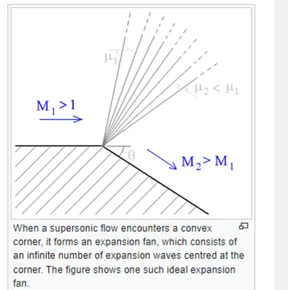
A supersonic expansion fan, technically known as Prandtl–Meyer expansion fan, a two-dimensional simple wave, is a cantered expansion process that occurs when a supersonic flow turns around a convex corner. The fan consists of an infinite number of mach waves, diverging from a sharp corner. When a flow turns around a smooth and circular corner, these waves can be extended backwards to meet at a point.

Shock wave

• Shock waves is generated when an object is moved faster than speed of sound (Supersonic Speed)
• And there is an abrupt change in the flow area or diversion, the flow process is irreversible and the entropy increases.
• Shock waves are very small regions in the gas where the gas properties change by a large amount.
• Across a shock wave, the static pressure, temperature and gas density increases almost instantaneously

Shock waves are of three types

Normal shocks: occurs when shock is 90 degrees (perpendicular) to the shock medium flow direction

Oblique shocks: occurs when shock is at certain angle to the shock medium flow direction

Bow shocks: occurs upstream of the front of a blunt object when the upstream flow velocity exceeds Mach 1.

Boundary conditions:

• Dirichlet boundary condition
• Neumann boundary condition

• Dirichlet boundary condition

In mathematics, the Dirichlet (or first-type) boundary condition is a type of boundary condition, named after peter Gustav Lejeune Dirichlet(1805–1859).When imposed on an ordinary or a PDE,s, it specifies the values that a solution needs to take along the Boundary of the domain.

• Neumann boundary condition

In mathematics, the Neumann (or second-type) boundary condition is a type of boundary condition, named after Carl Neumann When imposed on an ordinary or a PDE,s, the condition specifies the values of the derivative applied at the boundary of the domain.

Boundary condition in shock waves:
In case of shock flow problem Neumann boundary condition are used at the outlet. As outer boundary has no Influence on the inner nodes, in Neumann boundary conditions the values at the outlet is extrapolated from the inner nodes. Neumann boundary condition include derivate of the solution at the boundary

At the inlet Dirichlet boundary condition is provided. Dirichlet boundary condition specificizes the values that a solution needs to take along the boundary of the domain

Steps

• Imported STL file in converge studio
• Setup the case
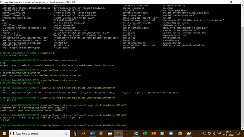
• Run the simulation in Cygwin
• Post process the results in PARAVIEW

Geometry

• Import STL files
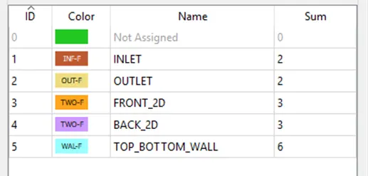
• Then give boundary flagging
• Then check normal transformation, all the face normal direction should be facing towards the flow region
• And finally, diagnosis

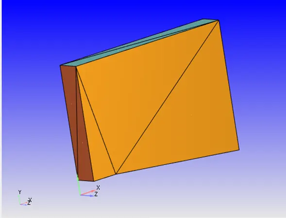
Click on boundary and Create boundary

Checking normal

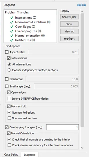
Before proceeding the error in geometry for that

View tab-diagnosis dock-default setting-select the find

Case Setup

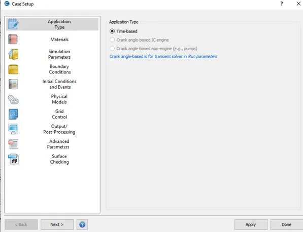
Application Type = Time-based

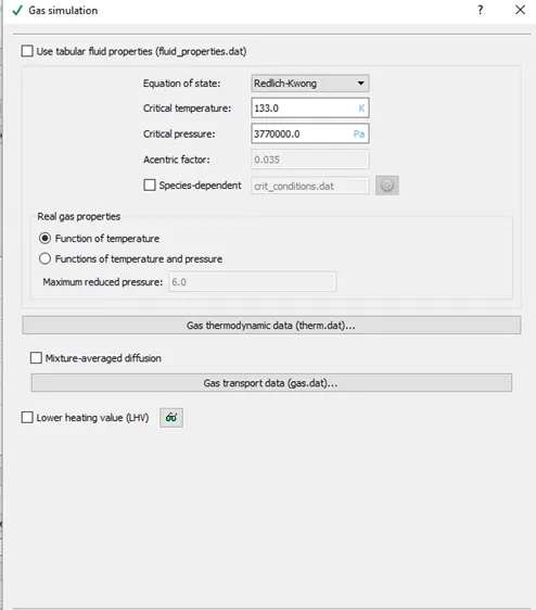
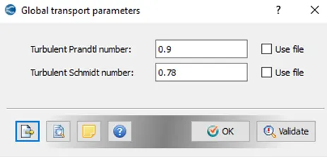
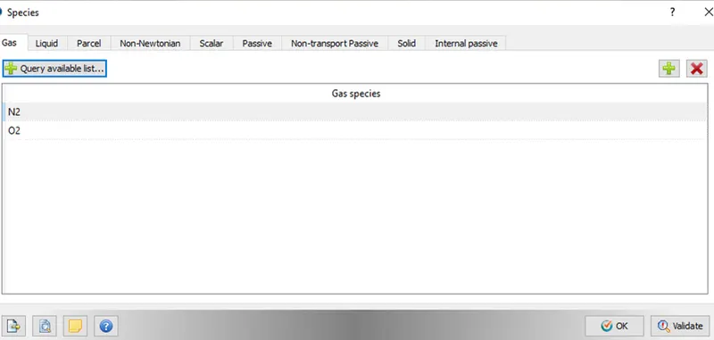
Materials -

Predefined mixtures = Air

Simulation Parameters-

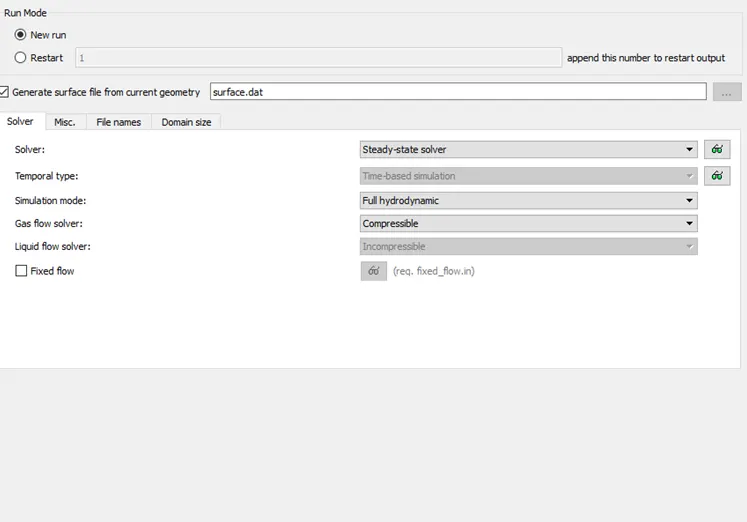
In Run Parameters two main things to be considered: -

select the following solver settings

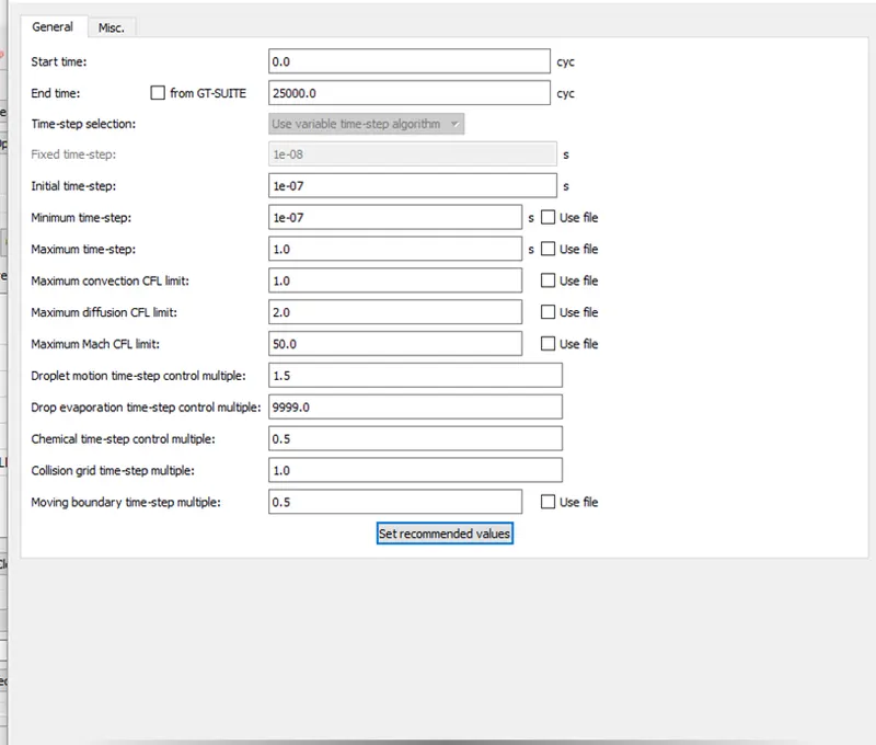
Simulation Time Parameters: -

Density based steady state solver

Start time-0

End time-25000 cycle

Initial time step-1e-07s

Minimum time step-1e-07s

Maximum time step-1s

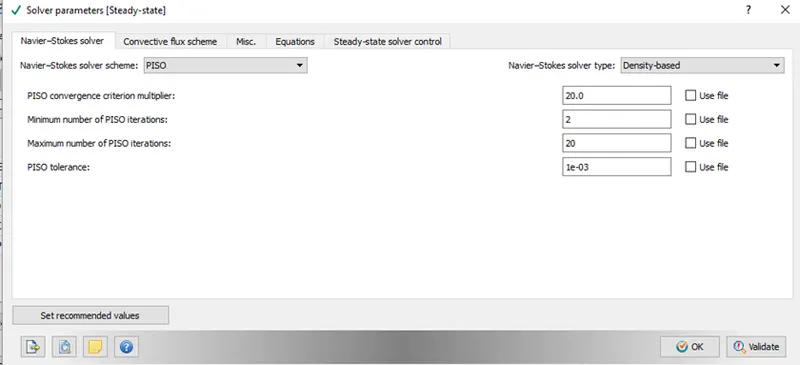
Solver Parameters [Steady-State]-

Navier-Strokes Solver type- Density based

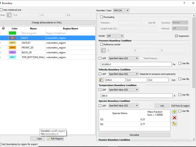
Boundary condition

Inlet-Inflow-

velocity-678m/s

pressure-101000pa

Temperature-286

Outlet-Outflow

Pressure -zero normal gradient

Velocity-zero normal gradient

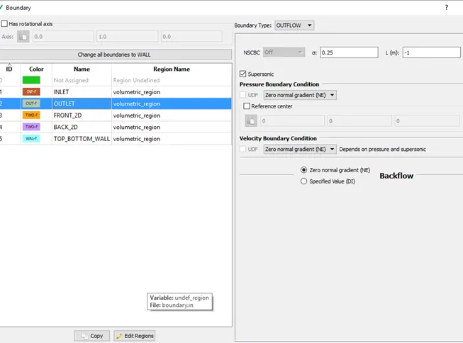
Front 2D

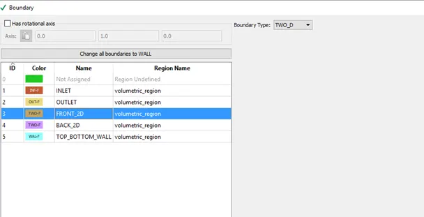
Back 2D

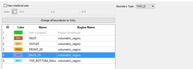
Top-bottom-wall-slip

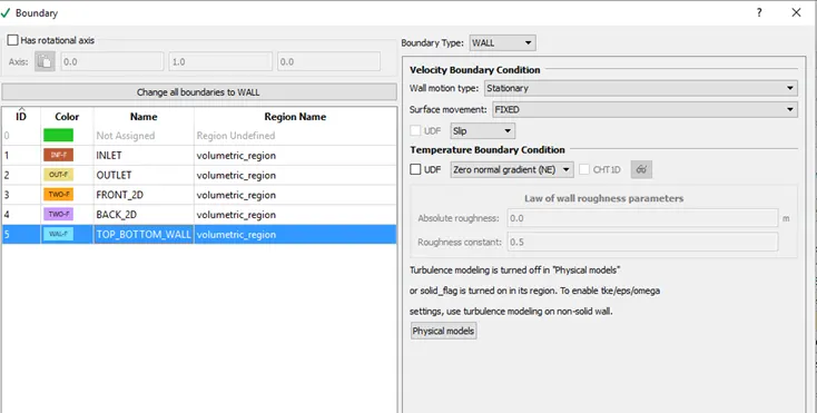
Turbulence modelling

Turbulence modelling- No need for turbulence modelling for this problem

In our simulation, we don’t have to use turbulence modelling since there is no Reynold stress because the flow is inviscid (viscosity is negligible)

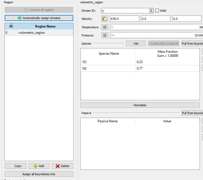
Region and initialisation

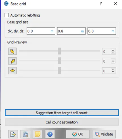
Base grid

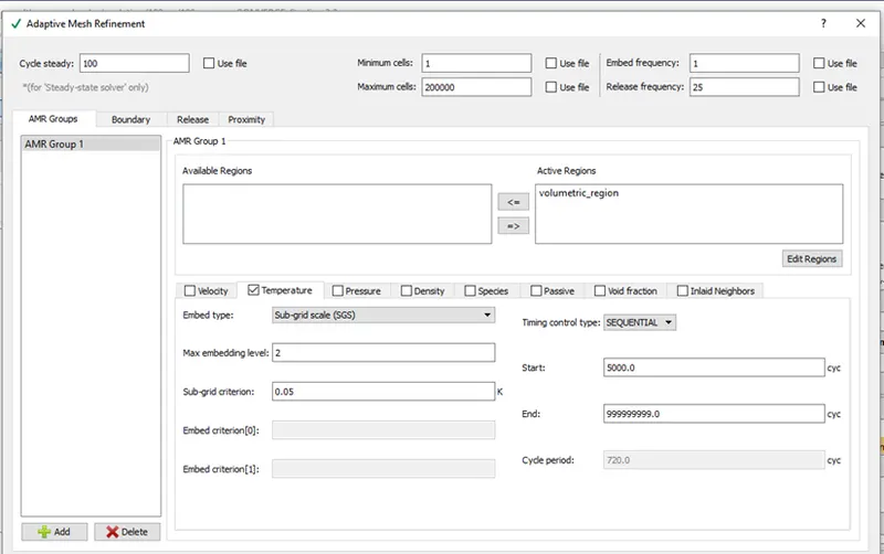
AMR (Adaptive mesh Refinement)

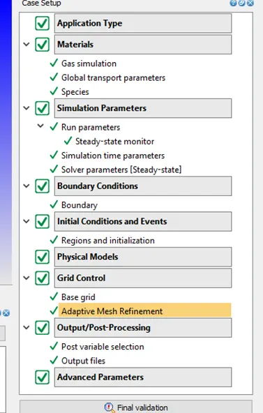
Note: check green tick mark on each option in case setup

Cygwin window

Results

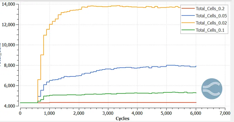
Cell Count

Total cell count for different SGS value

Case 1: SGS= 0.02k (Super-Sonic flow)

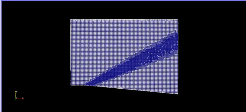
Mesh

For SGS 0.02 k the Adaptive mesh refinement is the maximum and mesh are very fine in shock region

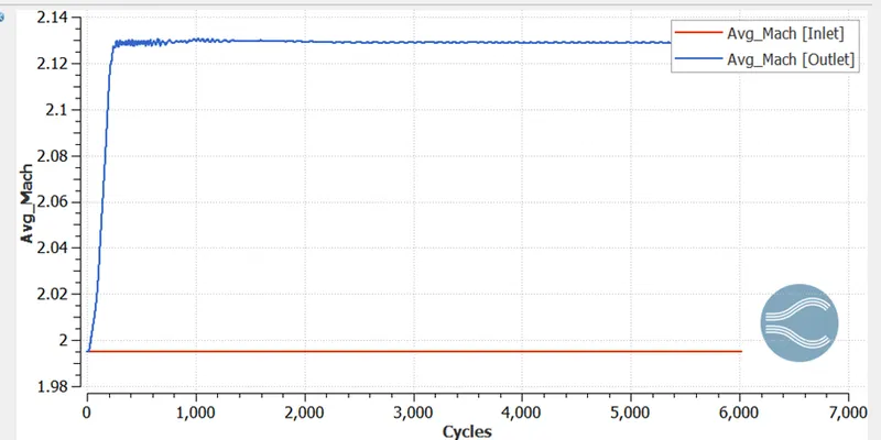
Mach number at inlet and outlet

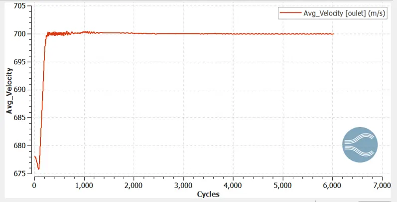
Velocity plot at outlet

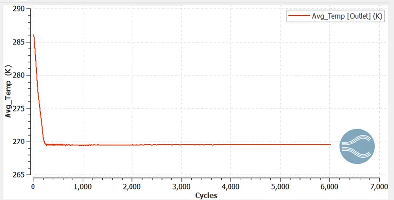
Temperature plot at outlet

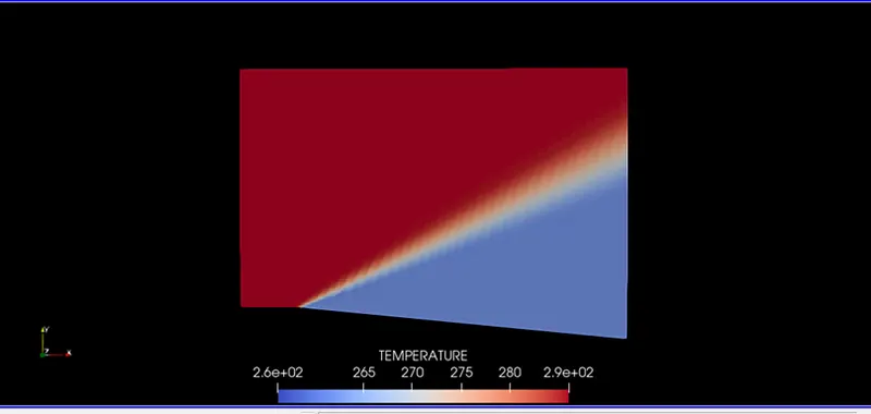
Temperature Contour

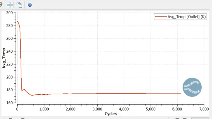
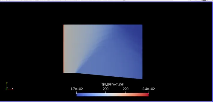
Temperature falls across the expansion wave i.e., T1>T2

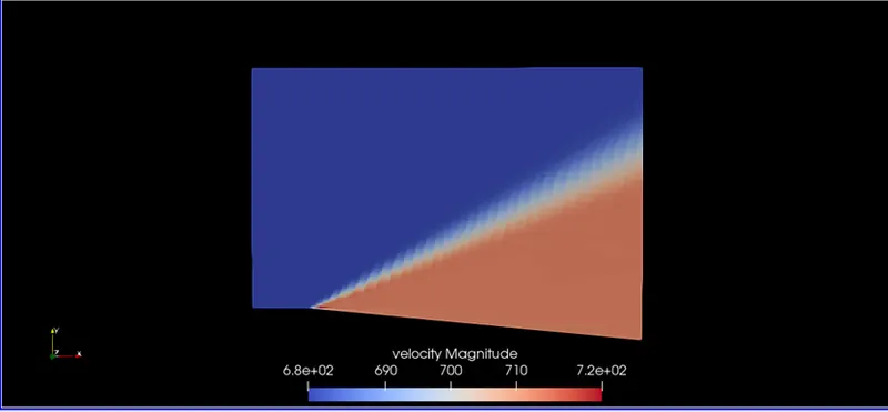
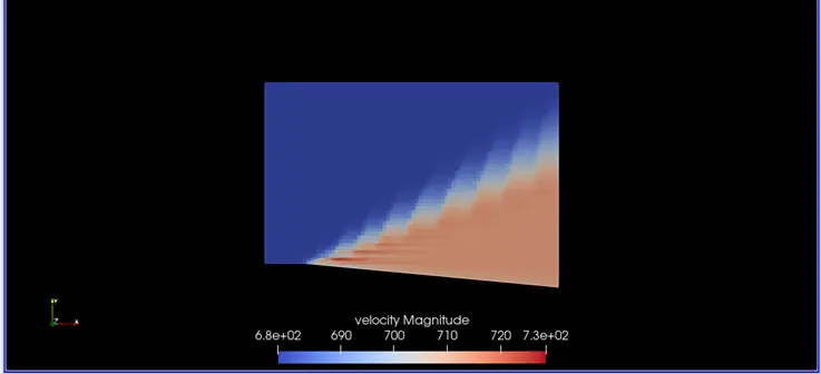
Velocity Contour

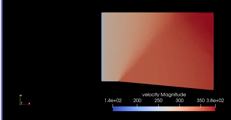
Velocity is increases across the expansion wave i.e., V1<V2

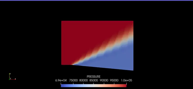
Pressure Contour

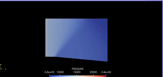
pressure falls across the expansion wave i.e., p1>p2

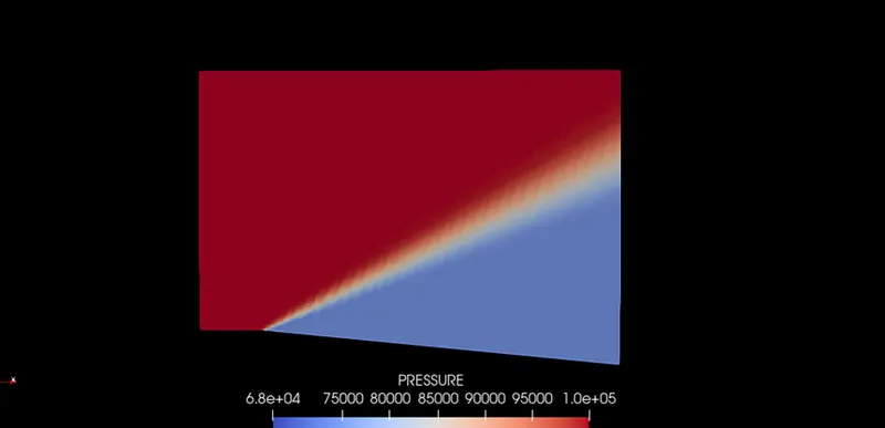
Case 2: SGS= 0.05k (Super-Sonic flow)

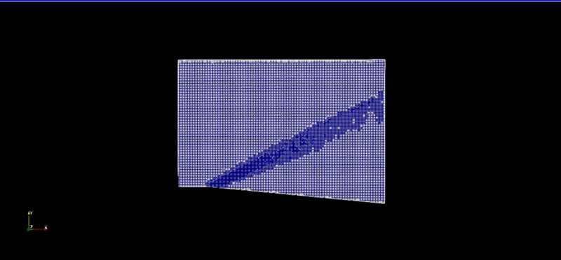
Mesh

For SGS-0.05K the Adaptive mesh refinement is less than the SGS 0.02

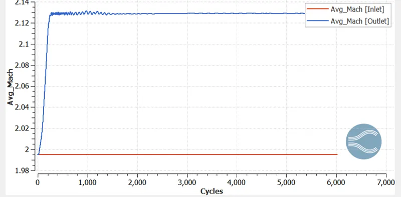
Mach number at inlet and outlet

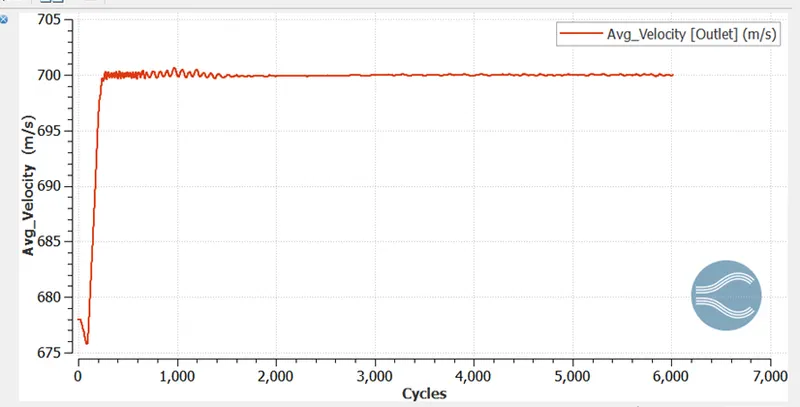
Velocity plot at outlet

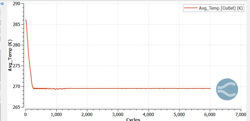
Temperature plot at outlet

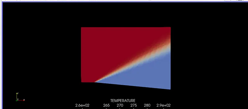
Temperature Contour

Temperature falls across the expansion wave i.e., T1>T2

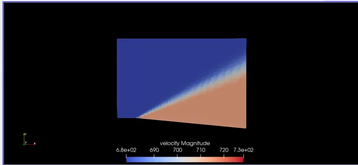
Velocity Contour

Velocity is increases across the expansion wave i.e., V1<V2

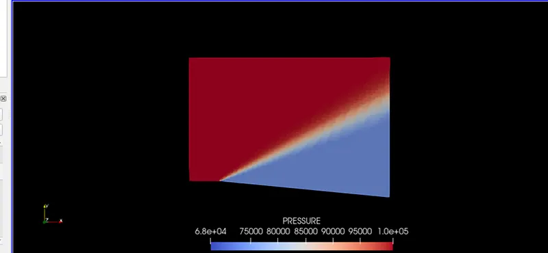
Pressure Contour

pressure falls across the expansion wave i.e., p1>p2

Case 3: SGS= 0.1k (Super-Sonic flow)

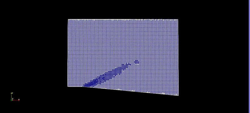
Mesh

For SGS-0.1K the Adaptive mesh refinement is less than the SGS 0.05 and the cell count is also less

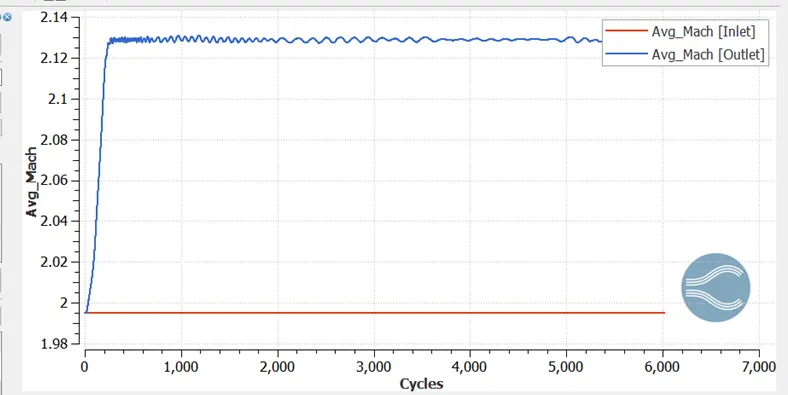
Mach number at inlet and outlet

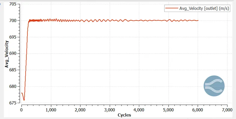
Velocity plot at outlet

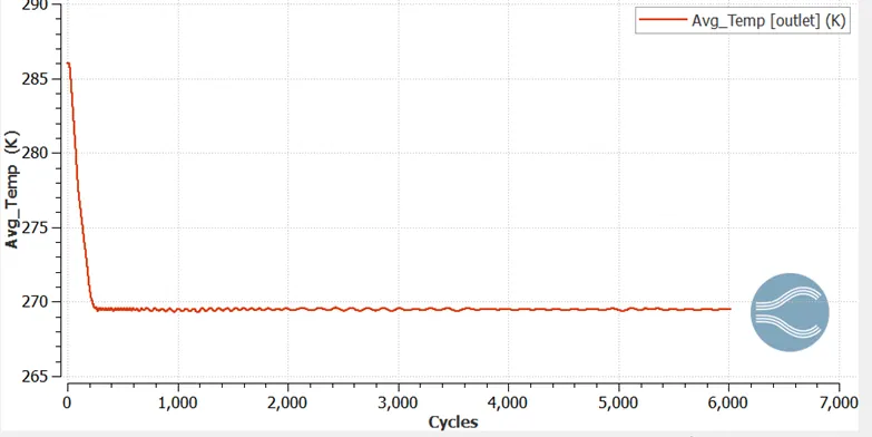
Temperature plot at outlet

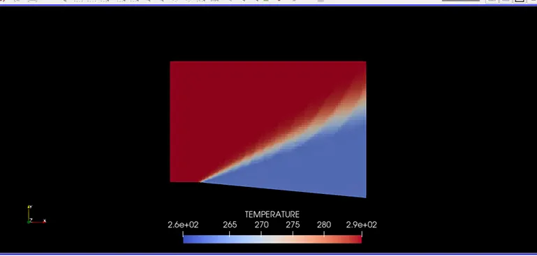
Temperature Contour

Temperature falls across the expansion wave i.e., T1>T2

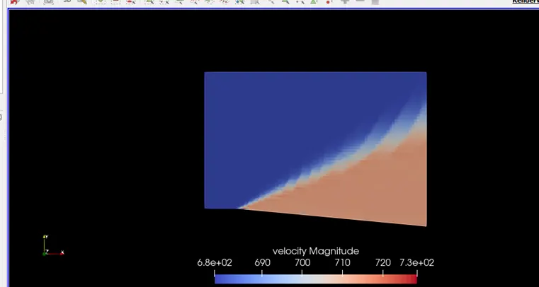
Velocity Contour

Velocity is increases across the expansion wave i.e., V1<V2

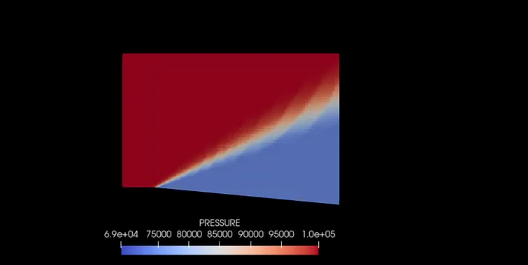
Pressure Contour

pressure falls across the expansion wave i.e., p1>p2

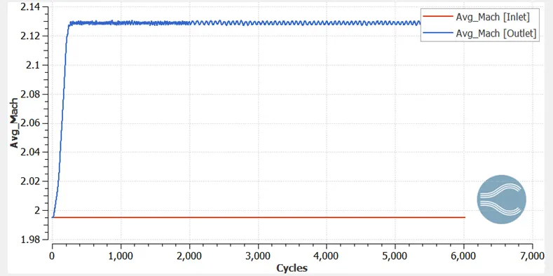
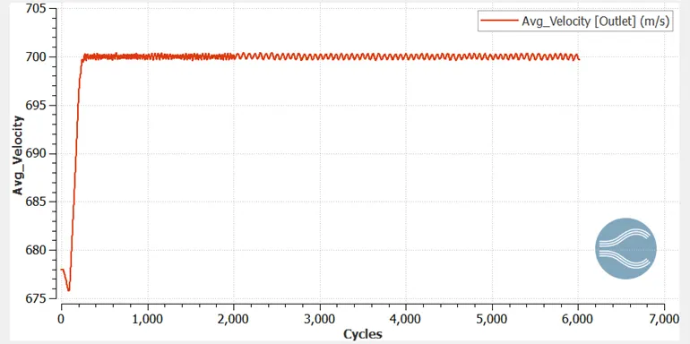
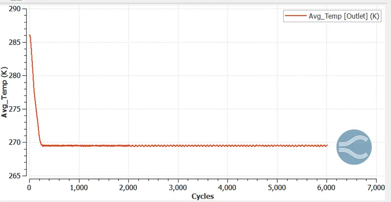
Case 4: SGS= 0.2k (Super-Sonic flow)

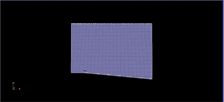
Mesh

For SGS-0.2K the Adaptive mesh refinement is less than the SGS 0.1 and the cell count is also less.The refinement criteria were so high that no refinement was achieved, it was as good as no adaptive mesh refinement.

Mach number at inlet and outlet

Velocity plot at outlet

Temperature plot at outlet

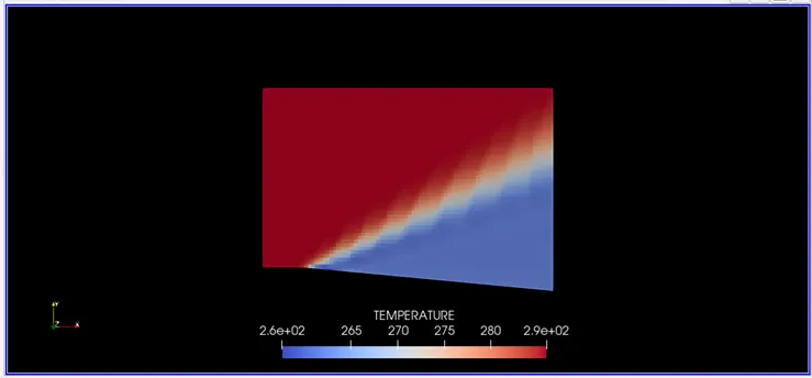
Temperature Contour

Temperature falls across the expansion wave i.e., T1>T2

Velocity Contour

Velocity is increases across the expansion wave i.e., V1<V2

Pressure Contour

pressure falls across the expansion wave i.e., p1>p2

Subsonic Case (AMR = 0.05)

Application Type = Time-based

Materials -

Predefined mixtures = Air

Boundary condition

Inlet-Inflow

Velocity -100m/s

pressure-101000pa

Temperature-286

Outlet-Outflow

Pressure and velocity – Zero normal gradient

Top and bottom wall- slip

Front and back- 2D

Cell count

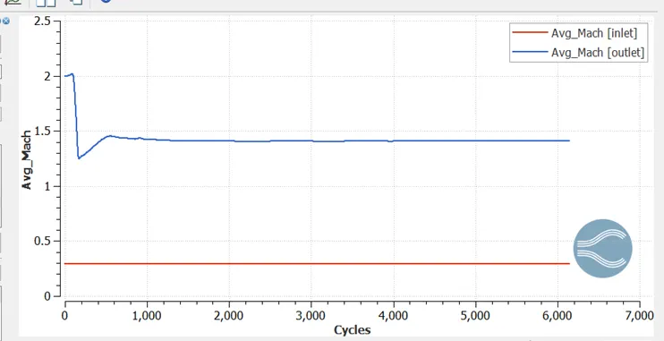
Mach number inlet and outlet

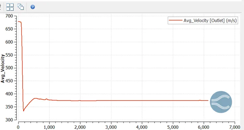
We can see Mach number increase from 0.3 to 1.5 across the shock wave indicating increasing velocity

Velocity plot

Temperature plot

Temperature contour

Velocity contour

Pressure contour

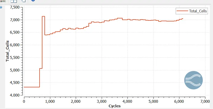
The effect of SGS temperature value on cell count and the shock location

From the above graph, the simulation with the least SGS value had the largest number of cell count. This is understandable because lower SGS ensures higher refinement and higher refinement results in higher number of cells.For SGS = 0.2, the refinement criteria were so high that no refinement was achieved, it was as good as no adaptive mesh refinement.

Video link

SGS 0.02k (Supersonic): -https://studio.youtube.com/video/BsbXxe59bqo/edit

SGS 0.05k (Supersonic): -https://studio.youtube.com/video/y_N1pbzX59I/edit

SGS 0.1k (Supersonic): -https://studio.youtube.com/video/Ot72Efp5A_Q/edit

SGS 0.2k (Supersonic): -https://studio.youtube.com/video/nO_INWRSiQA/edit

SGS 0.05K(Subsonic-100m/s):-https://studio.youtube.com/video/emqXazB1Yus/edit

Conclusions

• Prandtl mayor problem is run successfully for different SGS value
• With decreases SGS from 0.2 to 0.02 the number of cells count increased due to more mesh refinement
• With lower SGS criteria contour is smooth and results are more accurate