Week 5: Prandtl Meyer Shock problem

Prandtl-Meyer shock problem

• Aim:

To perform a steady state flow over a Prandtl-Meyer expansion fan, where the inlet velocity is having a Mach value of 2.0. Perform analysis using adaptive mesh refinement and the importance of sub-grid scale(SGS) at the flow separation region. Simulate for different values of SGS and post process the results.

• Introduction:

1. Mach number:

Mach number (M or Ma) is a dimensionless quantity in fluid dynamics representing the ratio of flow velocity past a boundary to the local speed of sound.

where:

M is the local Mach number,

u is the local flow velocity with respect to the boundaries (either internal, such as an object immersed in the flow, or external, like a channel), and

c is the speed of sound in the medium, which in air varies with the square root of the thermodynamic temperature.

By definition, at Mach 1, the local flow velocity u is equal to the speed of sound. At Mach 0.65, u is 65% of the speed of sound (subsonic), and, at Mach 1.35, u is 35% faster than the speed of sound (supersonic). Pilots of high-altitude aerospace vehicles use flight Mach number to express a vehicle's true airspeed, but the flow field around a vehicle varies in three dimensions, with corresponding variations in local Mach number.

The local speed of sound, and hence the Mach number, depends on the temperature of the surrounding gas. The Mach number is primarily used to determine the approximation with which a flow can be treated as an incompressible flow. The medium can be a gas or a liquid. The boundary can be traveling in the medium, or it can be stationary while the medium flows along it, or they can both be moving, with different velocities: what matters is their relative velocity with respect to each other. The boundary can be the boundary of an object immersed in the medium, or of a channel such as a nozzle, diffuser or wind tunnel channeling the medium. As the Mach number is defined as the ratio of two speeds, it is a dimensionless number. If M < 0.2–0.3 and the flow is quasi-steady and isothermal, compressibility effects will be small and simplified incompressible flow equations can be used.

2. Shock:

When the speed of the moving object in a medium becomes equal to the velocity of sound(340 m/s) in the medium, the wavefronts cannot escape from the source and pile up. This results in a large amplitude sound barrier. When the speed of the moving object or source exceeds the speed of sound in medium then the wavefronts lag behind the source forming a cone shaped region with a source at vertex. The edge of the cone forms a supersonic wave front with an unusually large amplitude called a shock wave. A sonic boom is heard when the shock waves reach an observer. The occurence of shock waves can be characterized by instantaneous change in pressure, velocity and temperature in a fluid flow. The region between the vehicle and the shock wave known as the shock layer will be a region of high pressure, density and temperature than the free-stream flow conditions. When a fluid streamline crosses the standing shock wave, abrupt increase in the pressure, temperature and density of the fluid flow occurs with a decrease in velocity of the flow.

3. Shock boundary conditions:

For solving the steady state flow appropriate boundary conditions are needed. It is one of the required components of the mathematical model. On the other hand, for solving transient flow, appropriate initial condition is also required. Boundary conditions are generally three types. They are Dirichlet boundary condition, Neumann boundary condition and mixed boundary condition. When using a Dirichlet boundary condition, the value of variable is prescribed at the boundary. Neumann boundary Conditions, When Neumann boundary Conditions imposed on an ordinary or a PDE, the condition specifies the values in which the derivative of a solution is applied within the boundary of the domain.

Pressure outlet boundary conditions require the specification of a static (gauge) pressure at the outlet boundary. The value of the specified static pressure is used only while the flow is subsonic. If the flow is supersonic, the specified pressure will no longer be used,pressure will be extrapolated from the flow in the interior. This means that Neumann Boundary Conditions which say that the outlet condition is dependent on the initial conditions of the flow need to be used in this case, that will derive the value of pressure from the initial conditions.

4. Prandtl-Meyer expansion fan:

A supersonic expansion fan, technically known as Prandtl–Meyer expansion fan, a two-dimensional simple wave, is a centered expansion process that occurs when a supersonic flow turns around a convex corner. The fan consists of an infinite number of Mach waves, diverging from a sharp corner. When a flow turns around a smooth and circular corner, these waves can be extended backwards to meet at a point.

Each wave in the expansion fan turns the flow gradually (in small steps). It is physically impossible for the flow to turn through a single "shock" wave because this would violate the second law of thermodynamics.

Across the expansion fan, the flow accelerates (velocity increases) and the Mach number increases, while the static pressure, temperature and density decrease. Since the process is isentropic, the stagnation properties (e.g. the total pressure and total temperature) remain constant across the fan.

• Case setup and simulation:

Performing the Prandtl-Meyer expansion fan under 4 different cases:

case 1: velocity=680 m/s, SGS= 0.005

case 2: velocity=680 m/s, SGS= 0.1

case 3: velocity=680 m/s, SGS= 0.8

csae 4: velocity=100 m/s, SGS=0.05

We'll perform 4 simulations to analyse the change in parameters when the SGS values are changed and also perform one simulation with subsonic inlet velocity and post process the changes derived on different cases.

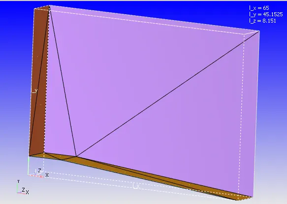
- Case setup:

1. Application type: time based

2. Materials:

a. Gas simulation: air

b. Global transport properties: Deafult

c. Species: O2 and N2

3. Simulation parameters:

a. Run parameters:

Steady-state solver, full hydrodynamic, compressible

b. Simulation time parameters:

- End time- 25000 cycles

- Time step- 1e-7

- min time step- 1e-7

- max time step- 1

- Convection CFL number- 0.5

c. Solver Parameters-

- Solver type- density based solver

- Equations- pressure- change preconditioner to none

- NS equations solver scheme: PISO

4. Boundary Conditions-

a. Inlet- Inflow

- Inlet velocity- 680 m/s

- Initial temp- 286.1K

- Species boundary condition- add air

b. Outlet- Outflow

Pressure: Zero normal gradient

Velocity: Zero normal gradient

Temperature backflow: Zero normal gradient

Species backflow: Mass fractions: Zero normal gradient

c. Top-bottom - Walls

slip condition- since we are not interested with the wall boundary physics and just the change in velocity, temperature, pressure and density.

d. Front and Back: 2D, since we are interested in performing a 2D simulation to save computational resource and simulation time.

5. Initial Conditions and Events:-

- Regions and Initialization:

Velocity: x-axis= 680 m/s, 100m/s

Pressure- 101325 Pa

Temperature: 286.1K

Add- air

6. Physical Models:-

- RNG k-epsilon

7. Grid Control:-

a. Base Grid:

dx = 0.3m, dy = 0.3m, dz = 0.3m

b. Addaptive mesh refinement:

- AMR with respect to Temperature

- Max embedding level: 2

- Sub-grid criterion(SGS): 0.05, 0.1, 0.8

- time control type: Sequential

- Start: 5000 , End: 999999999.0

Adaptive mesh refinement (AMR) is a method of adapting the accuracy of a solution within certain sensitive or turbulent regions of simulation, dynamically and during the time the solution is being calculated. When solutions are calculated numerically, they are often limited to pre-determined quantified grids as in the Cartesian plane which constitute the computational grid, or 'mesh'.

8. Post-Processing:-

- Post Variable Selection:

Select the parameters needed to be post processed.

- Output files:

We need to set a time interval for the files to be saved during each set of iterations. It is best suited to have a min of 100 saved files for every simulation. Therefore we need to calculate the time interval for writing the output files based on our end time given in run parameters.

Restart files help in restoring the files if there is a sudden power cut/ crash which is not helpful or might end up loosing the entire data, therefore the restart files helps in resuming the simulation form the point we lost contact. Restart files time interval can be same as the writing files interval which is safe and healthy.

In this case- since the end time is 25000, we can have a min of 100 so we have a interval to write the output after every 200 iterations. Therefore we have 125 output files.

• Results:

Base grid:

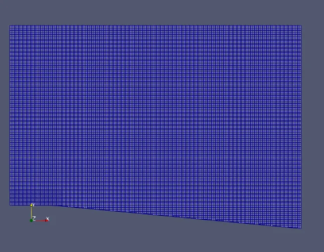
1. Case 1: v= 680 m/s, SGS=0.05

a. Mesh:

- Mesh grid:

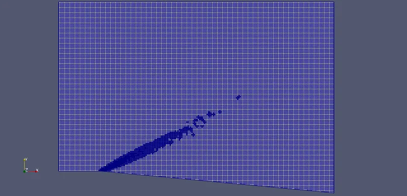
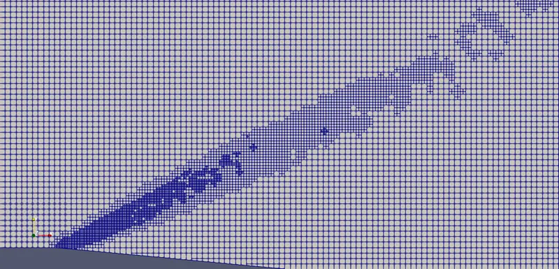
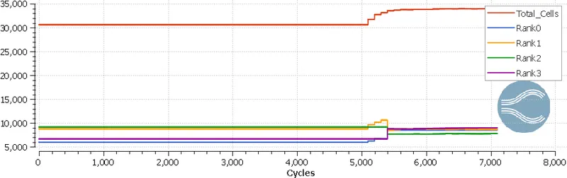
- Cell count:

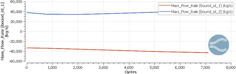
b. Mass flowrate:

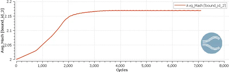
c. Mach number:

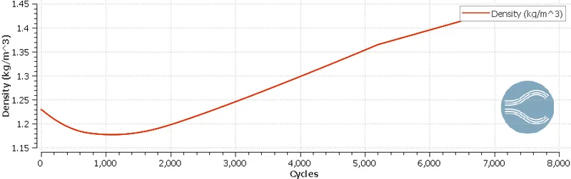
d. Density:

- Plot:

- Contour:

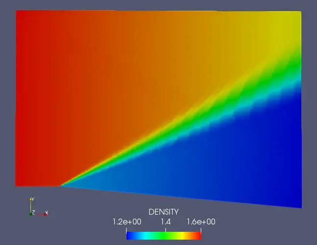
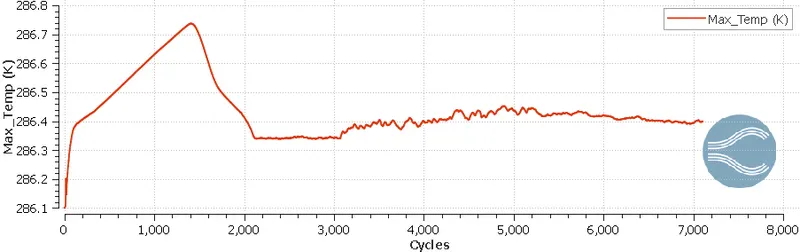
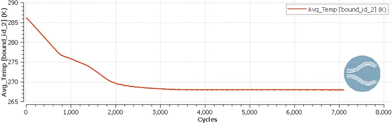
e. Temperature:

- Max temp:

- Average temperature:

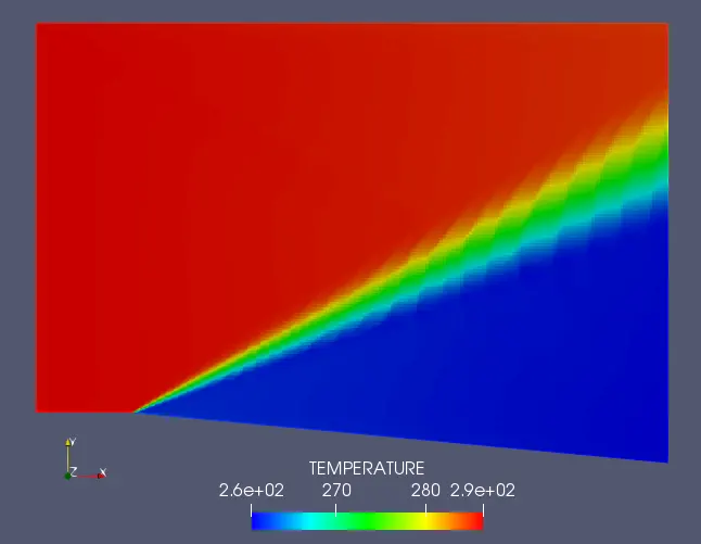
- Temperature contour:

f. Pressure:

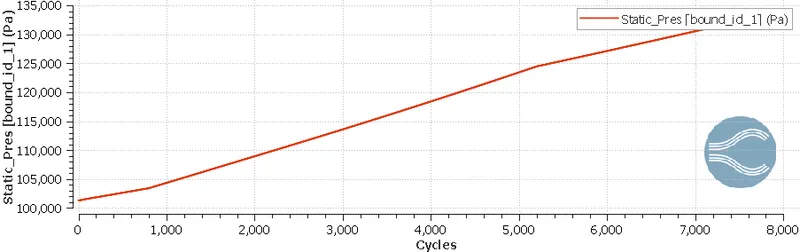
- Static pressure(inlet):

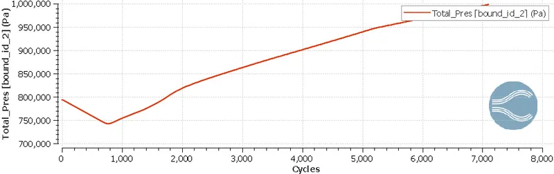
- Total pressure(outlet):

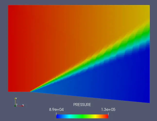
- Pressure contour:

g. Velocity:

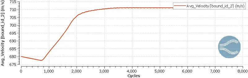
- Average velocity:

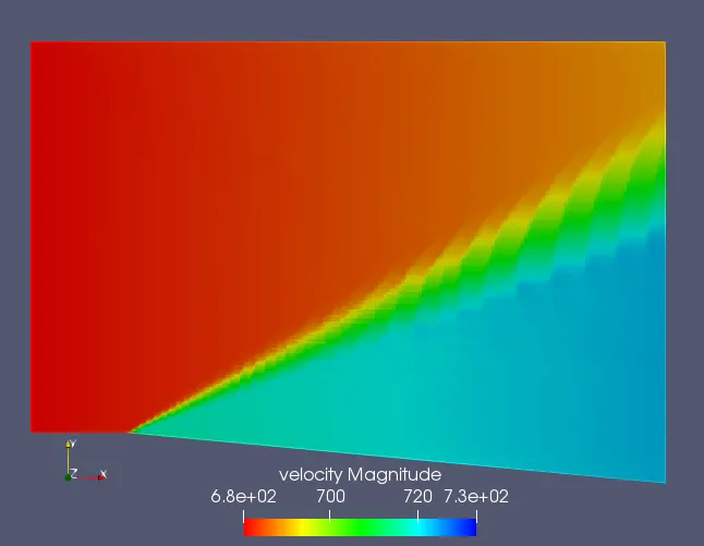
-Velocity contour:

h. Animations:

- Velocity:

- Temperature:

2. Case 2: v= 680 m/s, SGS=0.1

a. Mesh:

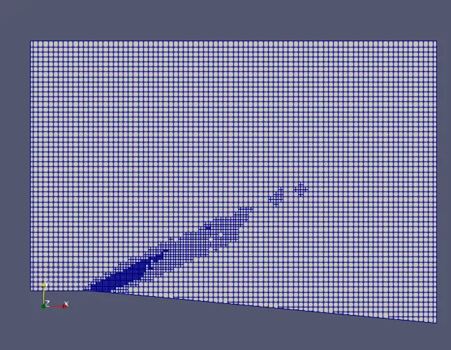
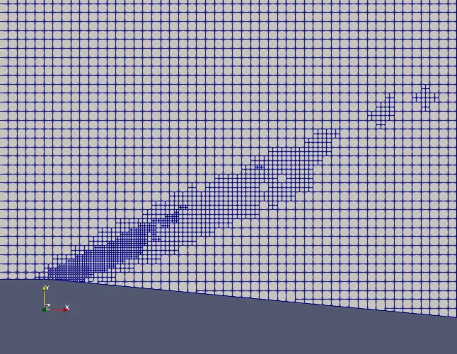
- Mesh grid:

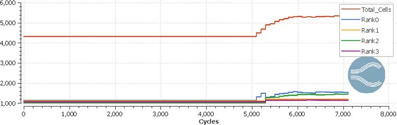
- Cell count:

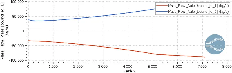
b. Mass flowrate:

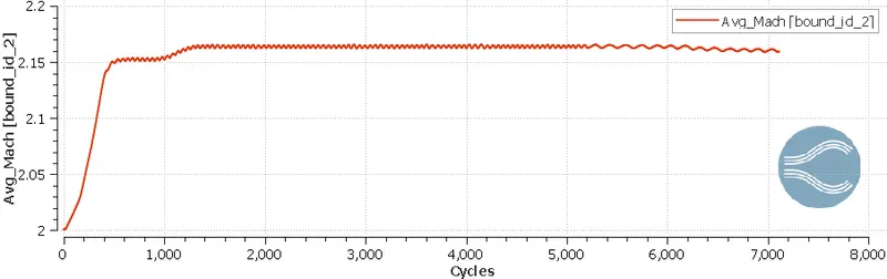
c. Mach number:

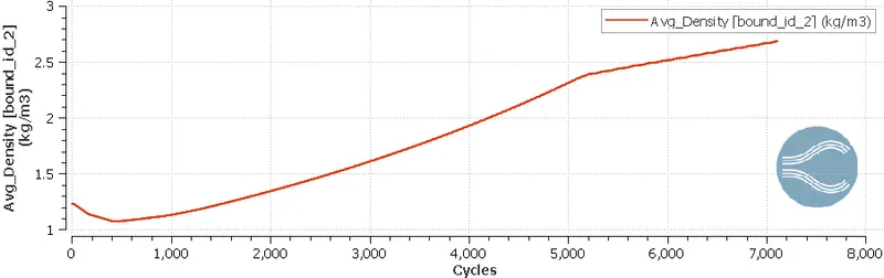
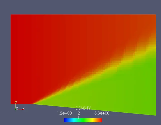
d. Density:

- Plot:

- Contour:

e. Temperature:

- Mean temperature:

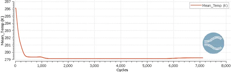
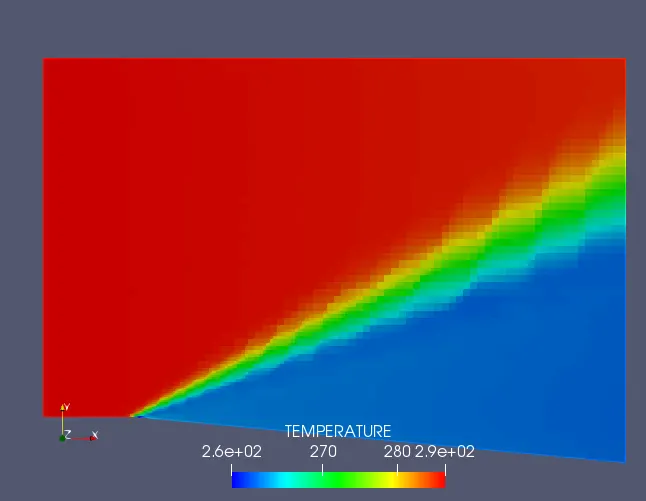
- Temperature contour:

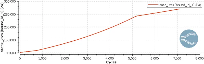
f. Pressure:

- Static pressure(inlet):

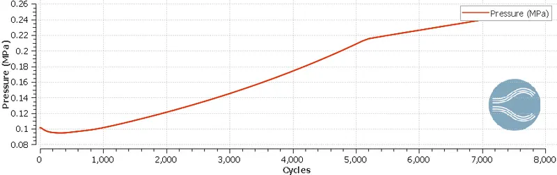
-Pressure:

- Pressure contour: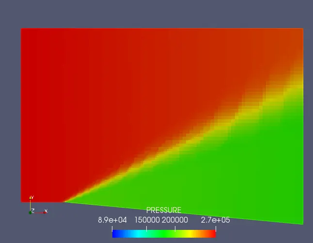

g. Velocity:

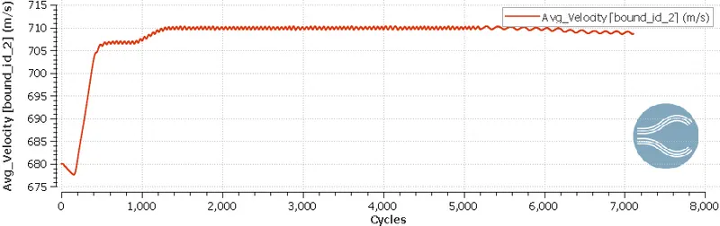
- Average velocity:

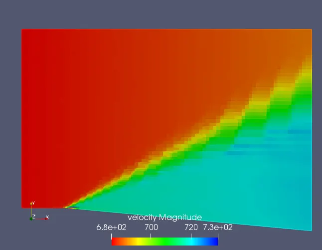
- Velocity contour:

h. Animations:

- Velocity:

- Temperature:

3. Case 3: v= 680 m/s, SGS=0.8

a. Mesh:

- Mesh grid:

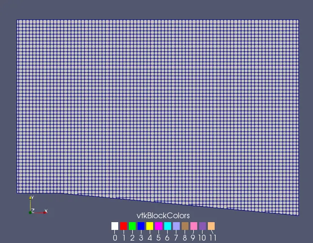
- Cell count:

b. Mass flowrate:

c. Mach number:

d. Density:

- Plot:

- Contour:

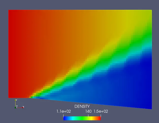
e. Temperature:

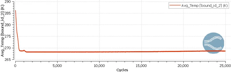
- Average temperature:

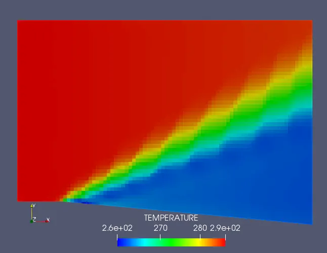
- Contour:

f. Pressure:

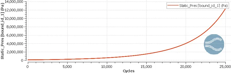
- Static pressure(inlet):

- Total pressure(outlet):

- Pressure contour:

g. Velocity:

- Average velocity:

- Velocity contour:

h. Animations:

- Velocity:

- Temperature:

4. Case 4: v= 100 m/s, SGS=0.05

a. Mesh:

- Mesh grid:

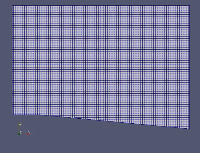
- Cell count:

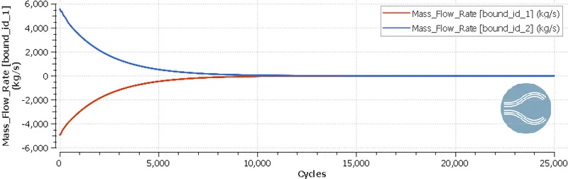
b. Mass flowrate:

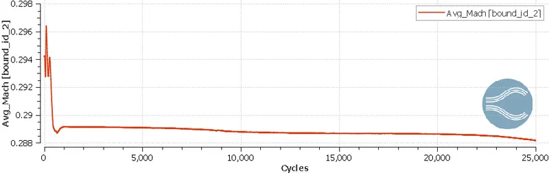
c. Mach number:

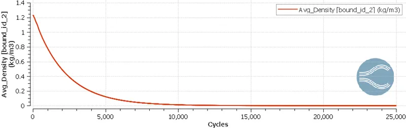
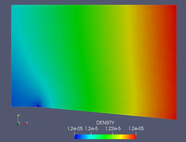
d. Density:

- Plot:

- Contour:

e. Temperature:

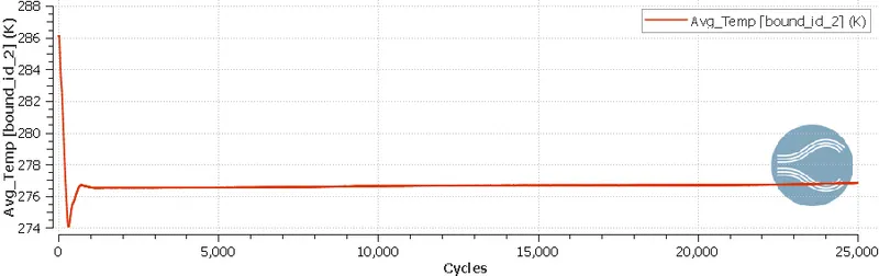
- Plot:

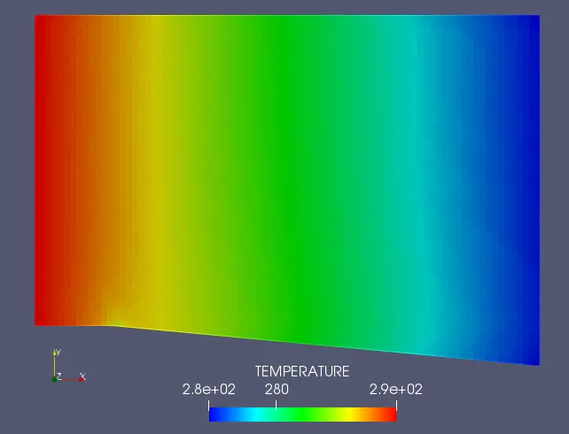
- Temperature contour:

f. Pressure:

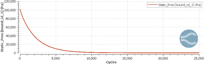
- Static pressure(inlet):

- Total pressure(outlet):

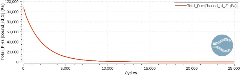
- Pressure contour:

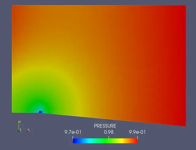
g. Velocity:

- Average velocity:

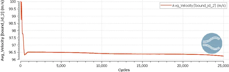
- Velocity contour:

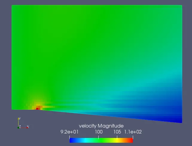
h. Animation:

- Velocity:

- temperature:

• Discussions:

1. It is evident that with an increase in the SGS criterion for temperature, the number of embedded cells decrease. This is because with an increase in the SGS criterion, the condition required for embedding new cells gets relaxed. Also the computational grids for Case 1 and Case 4 are same, since in both cases an SGS criterion of 0.05K is applied. At this point it can be easily predicted that the computational grid for Case 1 is best suited to capture the expansion fan as it can resolve the smallest temperature gradients among all grids.

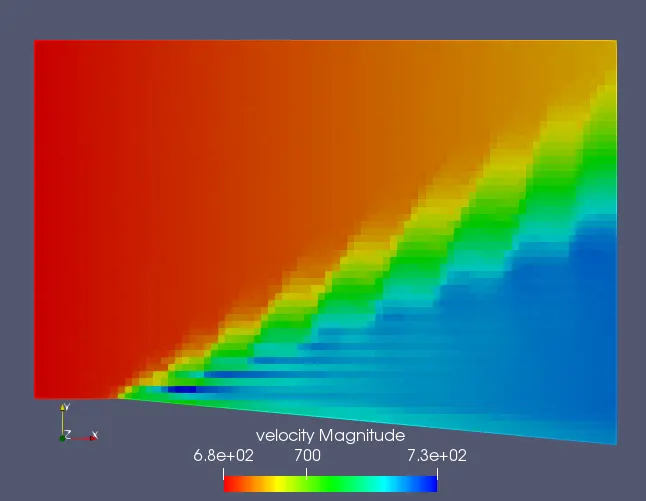
2. The plots show that across the expansion fan the air temperature is reduced. For all 3 cases, the expansion fan is located near the sharp corner but the tip of the fan is best resolved for Case 1, followed by Case 2 and Case 3 respectively. In other words, with an increase in the SGS criterion the resolution of the tip of the expansion fan decreases. There is minmal expansion in case 4 since the velocity is subsonic and doesn't play much difference in the expansion region.

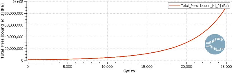
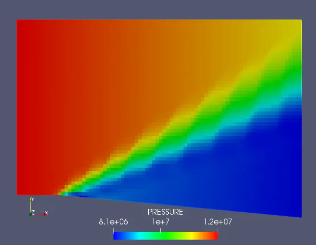
3. The plots show that across the expansion fan the air pressure is reduced. With an increase in the SGS criterion, the resolution of expansion fan decreases and it becomes more diffused. Also the pressure contours are almost the same for case 1, 2 and 3.

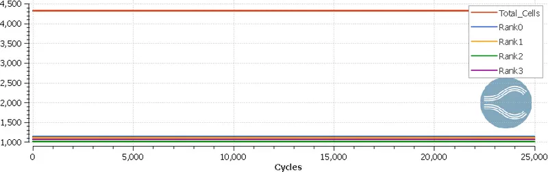
4. Since AMR is enabled, the total cell count changes with simulation cycles. Also the highest cell count is generated for Case 1 (and Case 4), as expected, followed by Case 2 and Case 3 respectively. In other words, the total cell count decreases with an increase in the SGS criterion.

5. AMR helps in refining the mesh effectively when we are in need of dealing with smaller grid sizes and also increasing the accuracy of the results obtained.

6. SGS helps in generating finer mesh as the SGS value is reduced and the contours appear blurred out when the SGS value is increased. Therefore its effective to use SGS to obtain better results and also improve the visibility of the contour.