Numerical simulation of Prandtl Meyer Shock phenomenon in a Supersonic flow field
I. Aim: Simulate Prandtl-Meyer shock waves using converge CFD.
II. Introduction:
In this project, the supersonic flow of air over a sharp corner is simulated using ConvergeCFD to study the Prandtl-Meyer shock (Expansion fan) phenomena. The case setup is done using ConvergeCFD and simulation is run in the CYGWIN terminal. Further, post-processing is done using ConvergeCFD and ParaView. The main objective of this project is to study the changes in flow properties like pressure, temperature, and Mach number changes after Prandtl-Meyer shock expansion.
Boundary conditions are boundaries in space for a dependent variable. A boundary condition expresses the behavior of a function on the boundary (border) of its area of definition.
The differential equation models for some of the phenomenon does not depend on time, such as a state of equilibrium. For this type of problems, a unique solution can be obtained by specifying conditions on the dependent variable on all the boundaries of the solution domain. Problems that require data on the entire boundary are called boundary value problems and the conditions at the boundary are called boundary conditions.
The common types of boundary conditions used in solving the flow differential equations (ordinary and partial) are:
1. Dirichlet Boundary condition:
A boundary condition that specifies the value of the function itself is a Dirichlet boundary condition.
example: `y(x1)=y1">y(x1)=y1y(x1)=y1`
here y is a function of x, and the value of y at x=x1 is y1. This type of boundary condition is called the Dirichlet boundary condition.
2. Neumann Boundary condition:
A boundary condition that specifies the value of the normal derivative of the function is a Neumann boundary condition or second-type boundary condition.
For example:
In the case of an insulated (infinitely thin) rod of length L, we can not have a heat flux beyond the ends so that the gradient of
the temperature must vanish (heat can only flow where a difference in temperature exists). This leads to the BC:
`(∂T)/(∂x)(0,t)=(∂T)/(∂x)(L,t)=0`
3. Mixed (Robin’s) Boundary Conditions:
It is the combination of both Dirichlet and Neumann boundary conditions. For the thin rod example above if we have the temperature at x=0 and time t is T(0,t) and T(L,t) at x= L and time t and the above Neumann boundary conditions, then:
`T ( 0 , t ) + (∂ T) /(∂ x) ( 0 , t ) = (∂ T) /(∂ x) ( L , t ) + T ( L , t ) = 0`
Boundary conditions for Shock flow problems:
1. Inflow Boundary condition:
In shock flow problems, the inflow boundary condition for the flow domain is defined in terms of the Dirichlet Boundary conditions (ie Specified Value) for all the flow properties.
Ex: In a supersonic flow involving a shock expansion, the velocity, Static Pressure, Temperature, etc are all defined in terms of specified values at the inflow boundary condition.
2. Outflow Boundary condition:
In shock flow problems, the outflow boundary condition for the flow domain is defined in terms of the Neumann Boundary conditions (ie zero normal gradients) for all the flow properties. This enables the flow properties to be computed at the outflow boundary during the solution depending on the changes occurring in the flow domain.
Ex: In a supersonic flow involving a shock expansion, the velocity, Pressure, Temperature, etc are all defined in terms of zero normal gradients. This enables the solver to compute these values depending on the flow changes in the domain due to shock waves generation.
3. Wall Boundary condition:
A shock wave occurs when the flow velocity exceeds the local sonic velocity (speed of sound). Usually, this occurs at high Reynolds numbers. At a high Reynolds number, the inertial forces are very large compared to that of the viscous forces. This makes the flow essentially inviscid. Hence slip occurs at any surface/wall in the flow. Therefore slip boundary condition is used at the surface/wall boundaries in a shock flow problem.
Shock Wave:
A shock wave or shock is a type of propagating disturbance that moves faster than the local speed of sound in the medium. Like an ordinary wave, a shock wave carries energy and can propagate through a medium but is characterized by an abrupt, nearly discontinuous, change in pressure, temperature, and density of the medium.
The energy and speed of a shock wave alone dissipate relatively quickly with distance. When a shock wave passes through matter, energy is preserved but entropy increases. This change in the matter's properties manifests itself as a decrease in the energy which can be extracted as work, and as a drag force on supersonic objects; shock waves are strongly irreversible processes.
Types of Shock waves:
- 1. Normal Shock: At 90° (perpendicular) to the shock medium's flow direction.
- 2. Oblique Shock: At an angle to the direction of flow.
- 3. Bow Shock: Occurs upstream of the front (bow) of a blunt object when the upstream flow velocity exceeds Mach 1.
Prandtl-Meyer Shock Wave ( Expansion Fan):
As an object moves through a gas, the gas molecules are deflected around the object. If the speed of the object is much less than the speed of sound of the gas, the density of the gas remains constant and the flow of gas can be described by conserving momentum and energy. As the speed of the objects increases towards the speed of sound, we must consider compressibility effects on the gas. The density of the gas varies locally as the gas is compressed by the object. When an object moves faster than the speed of sound, and there is an abrupt decrease in the flow area, shock waves are generated. If the flow area increases, however, a different flow phenomenon is observed. If the increase is abrupt, we encounter a centered expansion fan called Prandtl-Meyer Expansion fan.
Prandtl–Meyer expansion fan, is a two-dimensional shock wave that occurs when a flow at supersonic speed i.e. with a Mach no. greater than 1 turns around a sharp convex corner. as shown in the below figure:
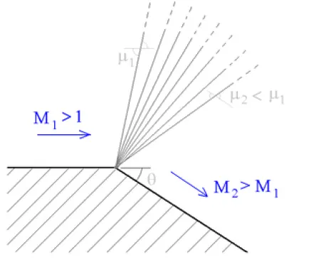
There are some marked differences between shock waves and expansion fans. Across a shock wave, the Mach number decreases, the static pressure increases, and there is a loss of total pressure because the process is irreversible. Through an expansion fan, the Mach number increases, the static pressure decreases, and the total pressure remain constant. Expansion fans are isentropic.
The calculation of the expansion fan involves the use of the Prandtl-Meyer function. This function is derived from the conservation of mass, momentum, and energy for very small (differential) deflections. The Prandtl-Meyer function is denoted by the Greek letter `nu` on the slide and is a function of the Mach number M and the ratio of specific heats `gamma` of the gas.
`nu = {sqrt[(gamma+1)/(gamma-1)]} * tan^-1{sqrt[(gamma-1)*(M^2 - 1)/(gamma+1)]} - tan^-1{sqrt[M^2 -1]}`
In this project, a 2D Prandtl-Meyer Expansion fan around a sharp corner in a supersonic flow is simulated and the effect of subgrid scaling of temperature values on total cell count and shock location is studied. The downstream flow properties are validated using an analytical solution.
III. Solving & Modelling approach:
2D steady-state CFD analysis of supersonic flow (Mach no. =2) over a sharp corner to simulate the Prandtl–Meyer expansion fan using ConvergeCFD case setup and then running the solution in CYGWIN terminal. Air is used as the fluid flowing over the sharp corner (77% N2 and 23% O2). Postprocessing is done using ConvergeCFD and ParaView.
1. Geometry/Domain:
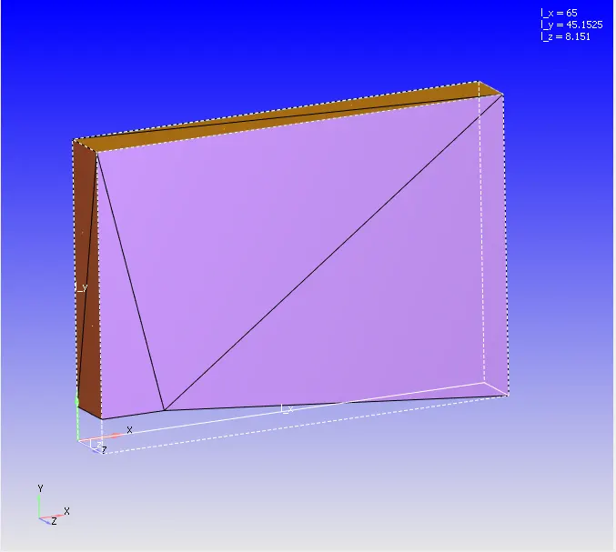
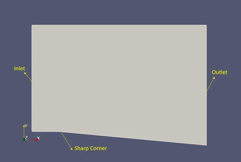
A 3D geometry with a typical sharp corner is imported into ConvergeCFD. The following figure shows the geometry. ConvergeCFD triangles are the basic building blocks. Hence the rectangular surfaces of the geometry are created using a combination of triangles. The bounding box dimensions of the geometry are also shown in the figure:
2. Boundary Flagging:
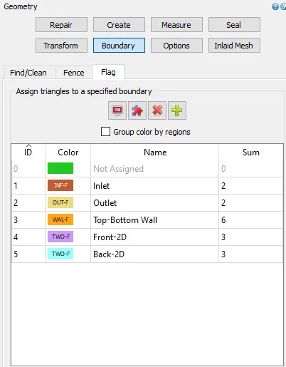
The boundary zones in ConvergeCFD are created by flagging boundaries. This can be done by creating boundary flags in the boundary tab as shown below:
3. Case setup:
After assigning boundary zones as mentioned above, the solution case setup is to be done. ConvergeCFD has a dedicated menu to completely set up the solution. Details are as follows:
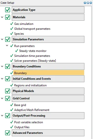
-In the application type option, Time-based is selected.
- The materials option are selected as shown in below images:
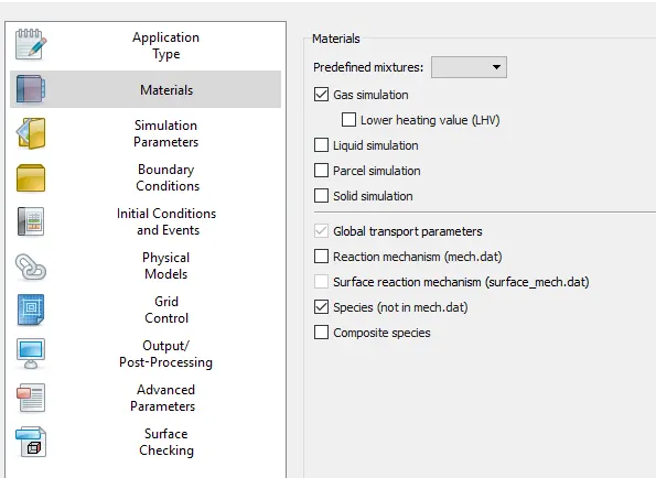
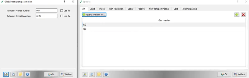
Air is chosen as the working fluid with 77% N2 and 23% O2.
- Simulation Parameters:
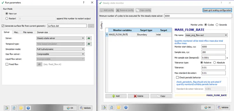
The steady-state solver option is selected and respective monitors for various flow variables are selected to monitor during the solution process.
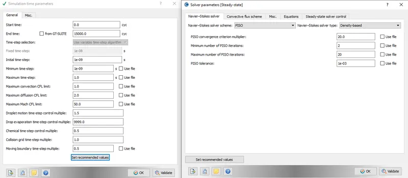
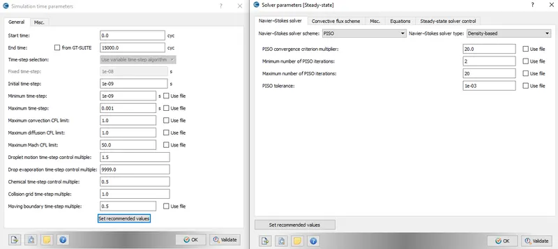
- Boundary Conditions:
The boundary conditions are assigned to the respective boundary zones in this menu. The applied boundary conditions are as follows:
| Boundary Zone | Boundary condition |
| Inlet |
Inflow (Dirichlet BC's) -Supersonic -Pressure = 101000 Pa, -Velocity = 678 m/s along x-direction -Temperature = 286 K - Species - O2 = 0.77, N2 - 0.23 |
| Outlet |
Outflow (Neuman BC's) - zero normal gradient Pressure - zero normal gradient Velocity -zero normal gradient backflow |
| Top-Bottom-wall |
Wall - Stationary, fixed, slip, zero normal gradient temperature. |
| Front-2D | TWO_D |
| Back-2D | TWO_D |
Since the flow is essentially 2D, the front and back faces of the domain are set to Two_D boundary conditions.
The above boundary conditions can be defined only after defining a region in the Initial conditions and Events section of the case setup as shown below:
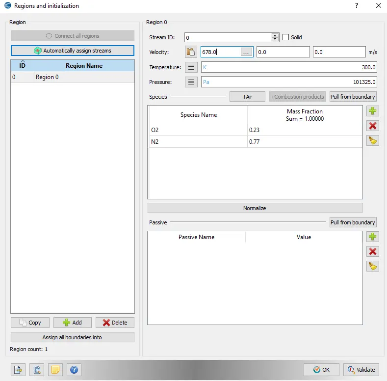
Turbulence is not considered in this analysis as the flow is essentially supersonic and inviscid.
- Grid control:
The base mesh size for the domain is defined in this tab as shown below:
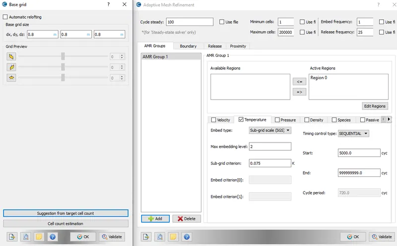
Also, the adaptive mesh refinement is turned on based on the sub-grid scaling (SGS) depending on the temperature variation sub-grid criterion in the flow domain as shown above.
The SGS temperature sub-grid criterion value effect on the cell count and shock location is studied for the following cases:
1. Temperature sub-grid criterion = 0.075
2. Temperature sub-grid criterion = 0.025
- Output and post-processing:
The flow variables of interest, which are to be post-processed after the solution are selected in this option ad also at how many intervals these are written to the output file.
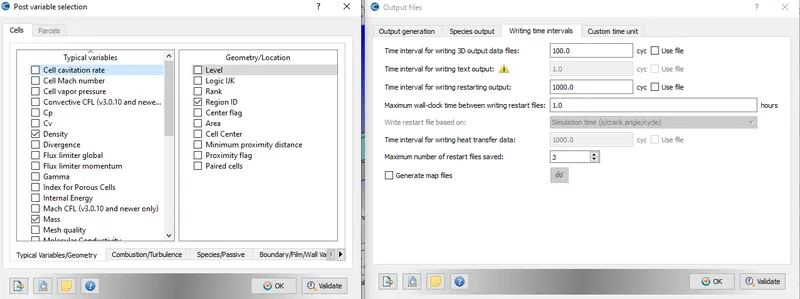
After all the above setup is completed final validation option is selected to check for the case setup is correct. After validation, the case setup files are exported using the export option in the File menu to the working folder. These files will be used by the CGYWIN terminal to run the solution. The above process is repeated for all the mesh sizes and the respective setup files are exported.
IV. Solution in CYGWIN :
The solution is run in the CYGWIN terminal. First, we have to navigate to the respective working folder in the CYGWIN terminal, where case setup files are present. Then by executing the following command, the solution can be run:
Navigating to folder:
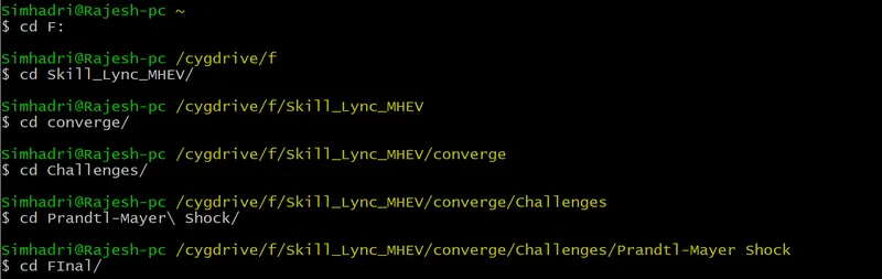

The solution will run-up to the number of cycles set in the run setup and the output files are saved to the respective folders.
V. Post-Processing Results:
After the solution is complete, post-processing of the results is done using CONVERGE CFD and ParaView.
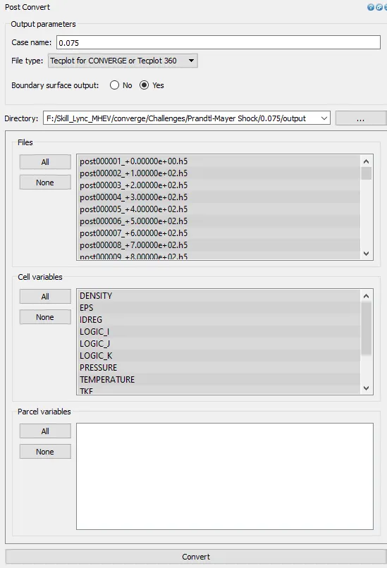
The plots are plotted in CONVERGE CFD, whereas to visualize the flow variables using contour plots the output files need to be converted to ParaView compatible files. This can be done in the CONVERGE CFD Post-Processing 3D tab as shown below:
Visualization in ParaView and graph plotting in Converge:
The converted ParaView compatible output files are opened in ParaView and the contour plots for Pressure, Temperature, and Velocity animation with mesh adaptment are visualized and graphs are plotted in converge as shown in below sections:
1. SGS with 0.075 sub-grid criterion for temperature value:
Total cell count:
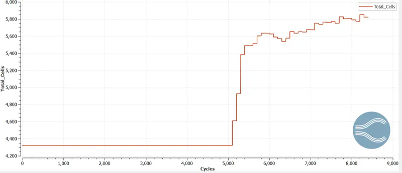
From the above plot, it can be seen that the mesh adaption starts after 5000 cycles according to the SGS criterion of 0.075 for temperature value.
Velocity Contour with adaptive mesh refinement:
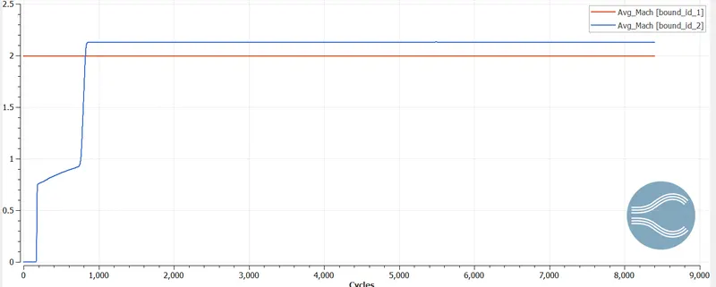
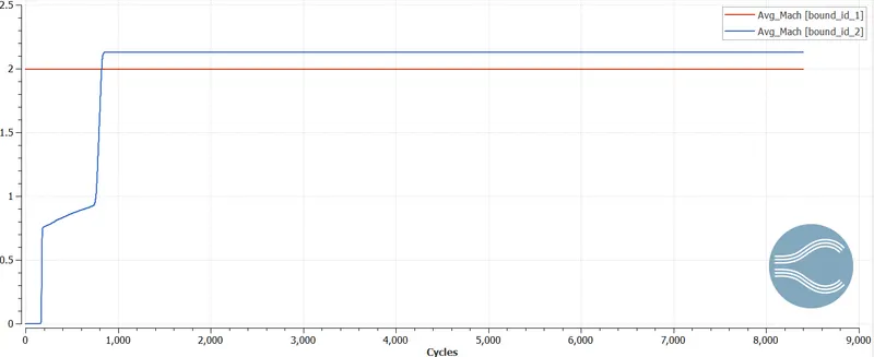
The above animation displays the Prandtl-Meyer Expansion Fan shock wave at a sharp corner. It can be seen the velocity increases from around Mach number, M=2 at upstream of the sharp corner to around Mach number, M=2.17 at downstream. Also, the grid adaption according to SGS criterion of temperature changes can be seen.
Pressure Contour:
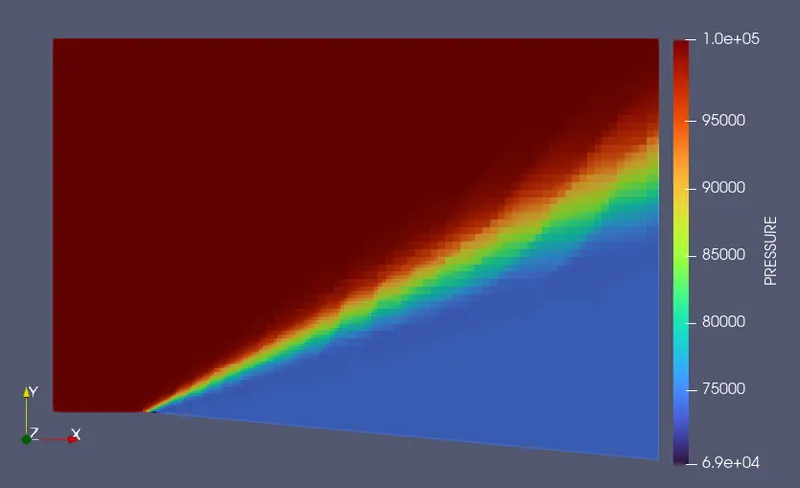
From the above contour plot, it can be seen that the pressure drops across the expansion wave (after the sharp corner) from 1 Bar at the upstream side to around 0.75 Bar on the downstream side. This is due to thermodynamic changes happening of flow accelerating to a higher Mach number in the Prandtl-Meyer Expansion fan.
Temperature Contour:
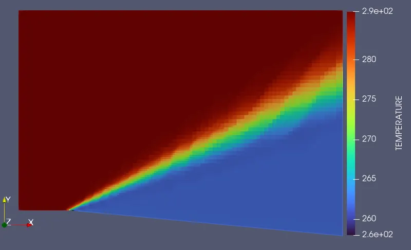
From the above contour plot, it can be seen that the Temperature drops across the expansion wave (after the sharp corner) from around 286 K at the upstream side to around 262 K on the downstream side. This is due to thermodynamic changes happening of flow accelerating to a higher Mach number in the Prandtl-Meyer Expansion fan.
2. SGS with 0.025 sub-grid criterion for temperature value:
Total cell count:
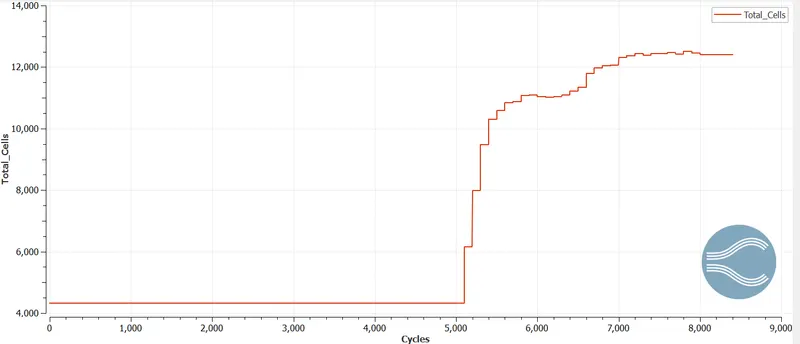
From the above plot, it can be seen that the mesh adaption starts after 5000 cycles according to the SGS criterion of 0.025 for temperature value.
Velocity Contour with adaptive mesh refinement:
The above animation displays the Prandtl-Meyer Expansion Fan shock wave at a sharp corner. It can be seen the velocity increases from around Mach number, M=2 at upstream of the sharp corner to Mach number, M=2.17 at downstream. Also, the grid adaption according to SGS criterion of temperature changes can be seen. The mesh refinement is more pronounced along the expansion fan in this case when compared to SGS 0.075 case.
Pressure Contour:
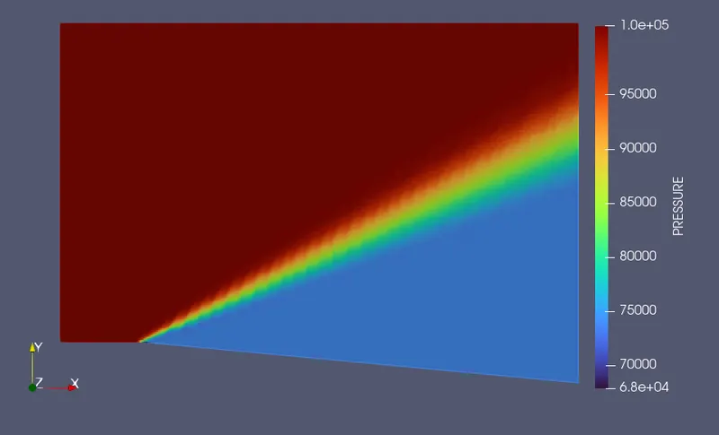
From the above contour plot, it can be seen that the pressure drops across the expansion wave (after the sharp corner) from 1 Bar at the upstream side to around 0.75 Bar on the downstream side. This is due to thermodynamic changes happening of flow accelerating to a higher Mach number in the Prandtl-Meyer Expansion fan.
Temperature Contour:
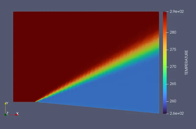
From the above contour plot, it can be seen that the Temperature drops across the expansion wave (after the sharp corner) from around 286 K at the upstream side to around 262 K on the downstream side. This is due to thermodynamic changes happening of flow accelerating to a higher Mach number in the Prandtl-Meyer Expansion fan.
Density Contour:
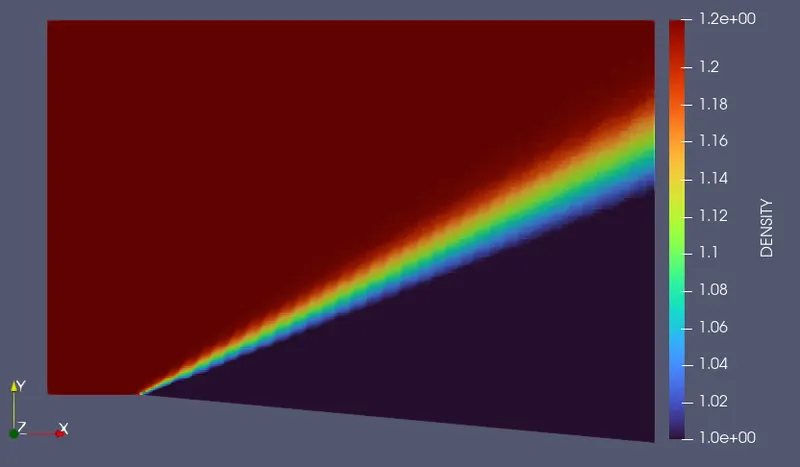
From the above contour plot, it can be seen that the density variations across the expansion wave (after the sharp corner) from 1.2 kg/m^3 at the upstream side to around 1.005 kg/m^3 on the downstream side. This is due to compressibility effects happening due to flow accelerating to a higher Mach number in the Prandtl-Meyer Expansion fan.
VI. Validation of Numerical solution with Analytical solution:
Analytical solution
1. Downstream Mach Number
The upstream conditions are:
Inlet Temperature, `T_1`=286 K,
Inlet Mach number `M_1`=3,
Inlet Pressure , `P_1`= 1.01 bar,
Inlet Density `rho_1` = 1.2 kg/m3
Other parameters:
Gamma=1.4 for air
corner angle,`theta`=5.352 degrees (measured from converge on the geometry)
The Prandtl-Mayer function `nu (M_1)` is given by the below formula at upstream Mach no. M1=2:
`nu = {sqrt[(gamma+1)/(gamma-1)]} * tan^-1{sqrt[(gamma-1)*(M^2 - 1)/(gamma+1)]} - tan^-1{sqrt[M^2 -1]}`
`nu (M_1) = sqrt((1.4-1)/(1.4+1))*tan^-1sqrt((1.4-1)/(1.4+1)*(2^2-1))-*tan^-1sqrt(3^2-1)`
`nu (M_1) = 49.756`degree`
The Prandtl-Mayer function `mu(M_2)` for the downstream condition is given by the turn angle formula :
`theta = nu (M_2)-nu (M_1)`
`nu (M_2) = theta+nu (M_1) = 5.352+26.452= 31.084 degrees`
The corresponding Mach number from the Prandtl-Mayer shock table [3].
`M_2` = 2.16
The above value when compared to the Mach number at the outlet from numerical simulation (around 2.17) is close enough.
2. Downstream Temperature
The Prandtl-Mayer expansion is an isentropic process, therefore:
`T_2/T_1=((1+(gamma-1)/2*M_1^2)/(1+(gamma-1)/2*M_2^2))`
`T_2=((1+(1.4-1)/2*2^2)/(1+(1.4-1)/2*2.1^2))*286 = 273.538 K`
3. Downstream Pressure:
`P_2/P_1=((1+(gamma-1)/2*M_1^2)/(1+(gamma-1)/2*M_2^2))^(gamma/(gamma-1))`
`P_2=((1+(1.4-1)/2*2^2)/(1+(1.4-1)/2*2.16^2))^(1.4/(1.4-1))*1.01= 0.786 Bar`
4. Downstream Density of fluid:
`rho_2/rho_1=((1+(gamma-1)/2*M_1^2)/(1+(gamma-1)/2*M_2^2))^(1/(gamma-1))`
`rho_2=((1+(1.4-1)/2*2^2)/(1+(1.4-1)/2*2.16^2))^(1/(1.4-1))*1.2=1.0039 (kg)/m^3`
The folowing table gives the comparison between numerical and analytical solution for downstream flow properties:
| Mach Number, M | Pressure (Bar) | Temperature (K) | Density (kg/m^3) | |
| A =Numerical | 2.17 | 0.75 | 262 | 1.005 |
| B = Analytical | 2.16 | 0.786 | 273.538 | 1.0039 |
| % Error = `|(A-B)/A|*100` | 0.46 | 4.58 | 4.21 | 0.11 |
From the above table, it can be seen that the numerical solution agrees well with the analytical solution with a maximum error of about 4.58%. Hence the numerical solution is validated with the analytical solution.
Conclusion:
In this project, the Prandtl-Meyer expansion fan shock phenomenon is simulated for a supersonic flow diversion along a sharp corner. The variation in the flow properties around the sharp corner due to the shock waves generated is studied numerically and the results are validated with analytical solution.
References:
1. https://www.grc.nasa.gov/www/k-12/airplane/pranmyer.html
2. https://en.wikipedia.org/wiki/Shock_wave
3. Modern Compressible flow with historical perspective by John D Anderson -Table A.5, Prandtl-Meyer function and Mach angle, page no.-710
4. https://skill-lync.com/knowledgebase/validation-of-prandtl-mayer-shock-problem