Week 5 - Mid term project - Solving the steady and unsteady 2D heat conduction problem

OBJECTIVE.

• To solve the 2D heat conduction equation by using the point iterative techniques for steady-state and Transient-state conditions.
• To write code for both implicit and explicit schemes (This is for the Transient Analysis only).

• For the Steady state, we have to solve it using three iterative approaches namely,

  1. Jacobi Method
  2. Gauss-Seidel Method
  3. Successive Over Relaxation Method.

  For the Transient state, we have to solve it using the same iterative methods but, in both Implicit and Explicit schemes.

GIVEN DATA.

The boundary conditions are given as follows,

Top Boundary = 600 K

Bottom Boundary = 900 K

Left Boundary = 400 K

Right Boundary = 800

2D Heat conduction Equation.

The heat equation is a second order partial differential equation that describes how the distribution of some quantity such as heat evolves over time in a solid medium, as it spontaneously flows from higher concentration area to lower concentration area.

Heat transfer is the transfer of thermal energy from a body, at a high temperature, to another at a lower temperature. This transfer of thermal energy may occur under steady or unsteady state conditions.

In this project, we will be solving the 2D heat conduction problem. But in reality, there is no such thing as 2 dimensional heat conduction, there is only 3D heat conduction. The 2D heat conduction analysis is generally done to observe the flow and its properties in 2D. And to understand the diffusion terms in the navier stokes equation.

FOR STEADY STATE AND TRANSIENT STATE HEAT CONDUCTION.

We have the 3D transient heat conduction

`(partial T)/(partial t) - alpha*((partial^2 T)/(partial x^2) + (partial^2 T)/(partial y^2)+(del^2T)/(delz^2) ) = 0`

this falls to 2D conduction equation as follows,

`(partial T)/(partial t) - alpha*((partial^2 T)/(partial x^2) + (partial^2 T)/(partial y^2))=0`

which is the transient state equation.

where,

`(partial T)/(partial t)` is the time derivative.

`(partial^2 T)/(partial x^2) + (partial^2 T)/(partial y^2)` is the spacial derivative.

`alpha` is the thermal diffusivity.

for the above transient equation applying the forward differencinng to the time derivative and applying the central differencing to the spacial derivative we get,

`T_(i,j)^(n+1)=T_(i,j)^n+alpha*(Deltat)/(Deltax^2)(T_(i-1,j)-2T_(i,j)+T_(i+1,j))^n+alpha*(Deltat)/(Deltay^2)(T_(i,j-1)-2T_(i,j)+T_(i,j+1))^n`

this is for the explicit method.

Applying forward differencing to the time derivative and central diffrencing to spacial derivative we get,

`T_(i,j)^(n+1)=T_(i,j)^n+alpha*(Deltat)/(Deltax^2)(T_(i-1,j)-2T_(i,j)+T_(i+1,j))^(n+1)+alpha*(Deltat)/(Deltay^2)(T_(i,j-1)-2T_(i,j)+T_(i,j+1))^(n+1)`

this can be written as,

`T_(i,j)^(n+1)=1/(1+2*k1+2*k2)(T_(i,j)^n+k1*(T_(i-1,j)+T_(i+1,j))^(n+1)+k2*(T_(i,j-1)+T_(i,j+1))^(n+1))`

where,

`k1=alpha*(Deltat)/(Deltax^2)`

`k2=alpha*(Deltat)/(Deltay^2)`

At steady state we have the equation,

`(partial^2 T)/(partial x^2) + (partial^2 T)/(partial y^2)=0`

By applying the central differencing scheme to the baove equation we get,

`(del^2T)/(delx^2)=(T_(i-1,j)-2T_(i,j)+T_(i+1,j))/(Deltax^2)`

and

`(del^2T)/(dely^2)=(T_(i,j+1)-2T_(i,j)+T_(i,j-1))/(Deltay^2)`

and then,

`T_(i,j)=(1/k)((T_(i-1,j)+T_(I+1,J))/(Deltax^2))+(1/k)((T_(i,j-1)+T_(i,j+1))/(Deltay^2))`

where,

`k=2*((Deltax^2+Deltay^2)/(Deltax^2*Deltay^2))`

we are using different iterative methods to solve in the implicit method for both steady state and unsteady/transient state conduction are as follows,

• JACOBI – IN this method, the 2D heat conduction equation solves using calculating the value of Temperature at inner nodes using several iterations, in which each value of temperature will be previously assigned temperature values at nodes.

• GAUSS-SEIDEL – In this method, the 2D heat conduction equation solves, we are calculating the value of temperatures at inner nodes using several iterations, in which every value of temperature will be updated successively with respect to the previous iteration.

• SUCCESSIVE OVER-RELAXATION- In this method, the 2D heat conduction equation solves. We are calculating the value of temperatures at inner nodes using several iterations, in which every value of temperature will be updated successively with respect to the previous iteration. And also “Relaxation factor” multiplies to the algebraic equation to alter the path of the iteration.

When Relaxation factor < 1 under relax

When Relaxation factor > 1 over relax

The value of Relaxation factor can be taken as 1.1 or 1.2

The Relaxation factor plays a vital role in determining the rate of convergence for CFD simulation.

PROGRAM LOGIC.

• We will start with the regular clear commands clear all, close all, clc.
• Assigning the inputs length in x direction and y direction and also taking the number of nodes nx and ny and creating the equally spaced grids by using the linspace command.
• and we need to show the y axis points in the reverse direction in the plot so we are using the 'fliplr' command to reverse the y direction plots.
• And then assigning the formula for k, k1 and k2 which we are using in the functions for the calculations.
• Taking the boundary conditions given as the initial guess values for the calculation and also assigning the tolerance value which is given and also taking the relaxation factor w as 1.2.
• And after this we are creating functions to compute for steady and unsteady state heat condutcion so that we can obtain the solutions for all the steady and unsteady state heat conduction plots in one run.
• For steady state conduction we are using the while loop which is convergence loop because we are calculating in the equillibrium state so we dont have time loop here and using while loop we are going to calculate for jacobi, Guass siedal, and Successive over relaxation methods for implicit method for steady stat econduction by creating three functions for three iterative solving methods. While loop will stops iterating when it reaches the convergence.
• And for unsteady state heat conduction also we are creating function for explicit method and for implicit method using the jacobi, Guass siedal, and successive over relaxation iterative methods we are supposed to create four functions for unsteady state heat conduction.
• For all the iterations we are plotting the graphs to observe how the diffusion is taking splace in case of heat conduction, which is converging here that can be observed in the graphs.
• and creating all the functions we need to call the functions that we can obtain the desired output.

CODE

Main program

clear all
close all
clc

% Inputs 
L=1;
H=1;
nx=10;
ny=10;
x=linspace(0,L,nx);
y=linspace(0,H,ny);
y=fliplr(y);
dx=x(2)-x(1);
dy=y(2)-y(1);

k=2*((dx^2+dy^2)/(dx^2*dy^2));
dt=(0.5/1.4)*((dx^2*dy^2)/(dx^2+dy^2));
k1=1.4*(dt/dx^2);
k2=1.4*(dt/dy^2);
CFL=1.4*(dt/dx^2);
[X,Y]=meshgrid(x,y);


% Initializing temperature
T=300*ones(nx,ny);
T(:,1)=400;
T(:,end)=800;
T(1,:)=600;
T(end,:)=900;
T_old=T;
nt=1400;
tol=1e-4;
error=1;
iter=0;
w=1.2;

% solving the steady state conduction equation by using jacobi iteration method
solver_1=fun_jacobi(error,tol,nx,ny,X,Y,dx,dy,T_old,T,k);

% solving the steady state conduction equation by using gauss siedal iteration method
solver_2=func_gauss_siedal(error,tol,nx,ny,X,Y,dx,dy,T_old,T,k);

% solving the steady state conduction equation by using successive over relaxation iteration method
solver_3=func_SOR(error,tol,nx,ny,X,Y,dx,dy,T_old,T,k,w);

% solving the unsteady state conduction by explicit method
explicit_method=fun_explicit(error,nx,ny,X,Y,dx,dy,T_old,T,k1,k2,dt,nt);

% solving the unsteady state conduction by implicit method by jacobi
% iterative method
transient_jacobi_method=func_transient_jacobi(nx,ny,X,Y,dt,dx,dy,k1,k2,T_old,T,tol,error,nt);

% solving the unsteady state by gauss siedal method
transient_GS_method=func_transient_GS(nx,ny,X,Y,dt,dx,dy,k1,k2,T_old,T,tol,error,nt);

% solving the unsteady state by SOR method
func_transient_SOR(nx,ny,X,Y,dx,dy,dt,error,nt,tol,k1,k2,w,T,T_old);

Functions created for the main program are,

Function for computing steady state heat conduction by implicit method by using jacobi iterative method.

function T=fun_jacobi(error,tol,nx,ny,X,Y,dx,dy,T_old,T,k)


iter=0;

while (error>tol)
    
    % space loop
    for i=2:nx-1
        
        for j=2:ny-1
            
            T(i,j)=(1/k)*(((T_old(i-1,j)+T_old(i+1,j))/(dx^2))+((T_old(i,j-1)+T_old(i,j+1))/(dy^2)));
        end
    end

 error=max(max(abs(T_old-T)));
    T_old=T;   % updating the T values
    iter=iter+1;

end
   figure(1)
    contourf(X,Y,T,'showText','on')
    xlabel('length')
    ylabel('heigth')
    title(sprintf('steady state heat conduction by jacobi method \n No of iteration:%d',iter))
end

Function for computing steady state heat conduction using guass siedal iterative method.

function T=func_gauss_siedal(error,tol,nx,ny,X,Y,dx,dy,T_old,T,k)

iter=0;
    while error>tol
    for i=2:nx-1
        
        for j=2:ny-1
            
            T(i,j)=(1/k)*(((T(i-1,j)+T_old(i+1,j))/dx^2+(T(i,j-1)+T_old(i,j+1))/dy^2));
            
        end
    end
    error=max(max(abs(T-T_old)));
    T_old=T;   % updating the T values
    iter=iter+1;
    
  
    end
    figure(2)
    contourf(X,Y,T,'showText','on')
    colorbar
    xlabel('length')
    ylabel('heigth')
    title(sprintf('steady state heat conduction by GS method \n No of iteration:%d',iter))

Function for computing the steady state heat conduction using SOR method.

function T=func_SOR(error,tol,nx,ny,X,Y,dx,dy,T_old,T,k,w)


    iter=0;
    tic
    while error>tol
    for i=2:nx-1
        
        for j=2:ny-1
            
            T(i,j)=(1-w)*T_old(i,j)+w*((1/k)*(((T(i-1,j)+T_old(i+1,j))/dx^2+(T(i,j-1)+T_old(i,j+1))/dy^2)));
            
        end
    end
    error=max(max(abs(T-T_old)));
    T_old=T;   % updating the T values
    iter=iter+1;
    
   
    end
   
       figure(3)
    contourf(X,Y,T,'showText','on')
    xlabel('length')
    ylabel('heigth')
    title(sprintf('steady state heat conduction by SOR method \n No of iteration:%d',iter))

Function for computing the transient heat conduction by explicit method.

function T=fun_explicit(error,nx,ny,X,Y,dx,dy,T_old,T,k1,k2,dt,nt)


% dt=(0.5/1.4)*((dx^2+dy^2)/(dx^2*dy^2));


    
for n=1:nt
    
    % space loop
    for i=2:nx-1
        
        for j=2:ny-1
            
            T(i,j)=T_old(i,j)+k1*(T_old(i-1,j)-2*T_old(i,j)+T_old(i+1,j))+k2*(T_old(i,j-1)-2*T_old(i,j)+T_old(i,j+1));
        end
    end

   
    T_old=T;   % updating the T values
 

end


    figure(4)
    contourf(X,Y,T,'showText','on')
    xlabel('length')
    ylabel('heigth')
    title('solving by explicit method for no of time step=1400')
   

Function for computing the transient conduction by using implicit method by jacobi iterative method.

function T=func_transient_jacobi(nx,ny,X,Y,dt,dx,dy,k1,k2,T_old,T,tol,error,nt)

T_guess= T_old;
Term_1=(1+2*k1+2*k2)^-1;
Term_2=(k1*Term_1);
Term_3=(k2*Term_1);

iter=0;
tic
% time loop
for n=1:nt


error=1;
    % convergence loop
    while error>tol
        
        % space loop
        for i=2:nx-1
            for j=2:ny-1

                T(i,j)=Term_1*T_old(i,j)+Term_2*(T_guess(i-1,j)+T_guess(i+1,j))+Term_3*(T_guess(i,j-1)+T_guess(i,j+1));
            end
        end
        error=max(max(abs(T_guess-T)));
        T_guess=T;
        iter=iter+1;
       
    end
    T_old = T;
    
end
    time_trans_jacobi=toc  
    figure(5)
    contourf(X,Y,T,'showText','on')
    xlabel('length')
    ylabel('heigth')
    title(sprintf('solving for transient conduction \n by jacobi\n no of iterations = %d',iter))

Function for computing the transient heat conduction by guass siedal iterative method.

function T=func_transient_GS(nx,ny,X,Y,dt,dx,dy,k1,k2,T_old,T,tol,error,nt)

T_guess= T_old;
Term_1=(1+2*k1+2*k2)^-1;
Term_2=(k1*Term_1);
Term_3=(k2*Term_1);

iter=0;
tic
% time loop
for n=1:nt


error=1;
    % convergence loop
    while error>tol
        
        % space loop
        for i=2:nx-1
            for j=2:ny-1

                T(i,j)=Term_1*T_old(i,j)+Term_2*(T(i-1,j)+T_guess(i+1,j))+Term_3*(T(i,j-1)+T_guess(i,j+1))
            end
            
        end
        error=max(max(abs(T_guess-T)));
         T_guess=T;
        iter=iter+1;
       
    end
    T_old = T;
    
end
  time_trans_GS=toc  
    figure(6)
    contourf(X,Y,T,'showText','on')
    xlabel('length')
    ylabel('heigth')
    title(sprintf('solving for transient conduction \n by Gauss siedal\n no of iterations = %d',iter))

Function for computing the transient heat conduction by using SOR method.

function T=func_transient_SOR(nx,ny,X,Y,dx,dy,dt,error,nt,tol,k1,k2,w,T,T_old)

T_guess= T_old;
Term_1=(1+2*k1+2*k2)^-1;
Term_2=(k1*Term_1);
Term_3=(k2*Term_1);

iter=0;
tic


for n=1:nt
    
    error=1;
    while error>tol
        
   for i=2:nx-1
       
       for j=2:ny-1
           
           T(i,j)=(1-w)*T_guess(i,j)+w*(Term_1*T_old(i,j)+Term_2*(T(i-1,j)+T_guess(i+1,j))+Term_3*(T(i,j-1)+T_guess(i,j+1)));
           
       end
       
   end
   
   error=max(max(abs(T_guess-T)));
   T_guess=T;
   iter=iter+1;
   
    end
    T_old=T;
    
end

time_trans_SOR=toc

figure(7)
contourf(X,Y,T,'showText','on')
colorbar
xlabel('length')
ylabel('height')
title(sprintf('Transient heat conduction \n by SOR method\n No of iterations=%d',iter))

OUTPUT

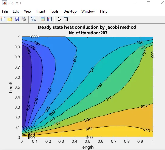
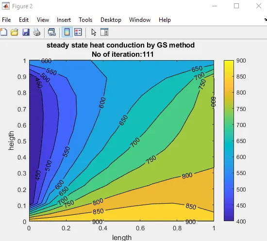
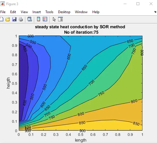
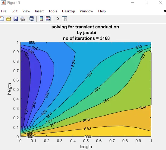
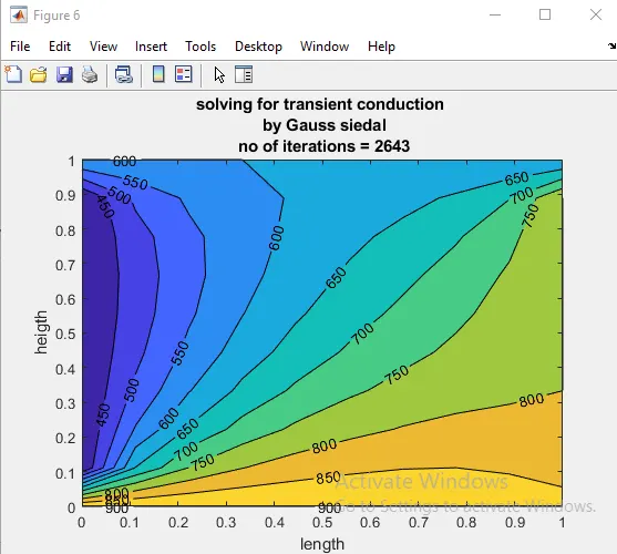
Here we can observe that number of iterations are reducing with the different iterative solver methods that is number of iterations in jacobi method>Guass siedal method>Successive over relaxation method.

Plot for steady state heat conduction using jacobi iterative solver method.

Plot for steady state heat conduction using Guass siedal iterative method.

Plot for steady state heat conduction using Successive over relaxation iterative method.

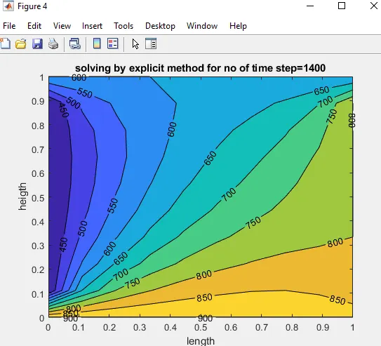
Plot for Unsteady state heat conduction using Explicit method.

Plot for Unsteady state heat conduction by using implicit method by jacobi iterative method.

Plot for Unsteady state heat conduction by usingn implicit method by guass siedal iterative method.

Plot for Unsteady state heat conduction by usingn implicit method by SOR iterative method.

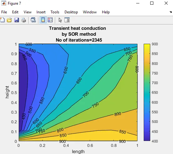
CONCLUSION.

From this we can observe that how the different iterative solver methods reduces the time in computing and reduces the number of iterations. Here number of iterations and time taken for computing jacobi method is greater than guass siedal method and number of iterations in guass siedal method are greater than successive over relaxation method. We can conclude that time taken for computation is Jacobi>Gauss Seidel>Successive Over Relaxation Method.