Week 3 - Taylor table method and Matlab code

OBJECTIVE

• To Derive the following 4th order approximations of the second-order derivative. 

         1. Central difference

         2. Skewed right-sided difference

         3. Skewed left-sided difference

• To write a program in Matlab to evaluate the second-order derivative of the analytical function `e^(x)*cos(x)` and to compare it with the 3 numerical approximations that we have derived.

Given data:

• Function, f(x)=`e^(x)*cos(x)`

EQUATIONS USED.

• Analytical second-order derivative,`f''(x)=-2*e^x*sin(x)`
• Central difference=`((m*(f(x-2*dx))+n*f(x-dx)+o*f(x)+p*f(x+dx)+q*f(x+2*dx)))/dx^2`

      In this case, we have the equation for the given function as follows and we have split it into terms to avoid mistakes. 

       t1=m*exp(x-(2*dx(i))).*cos(x-(2*dx(i)));
       t2=n*exp(x-dx(i)).*cos(x-dx(i));  
       t3=o*exp(x).*cos(x);
       t4=p*exp(x+dx(i)).*cos(x+dx(i));
       t5=q*exp(x+(2*dx(i))).*cos(x+(2*dx(i)));

       central_differencing=`(t1+t2+t3+t4+t5)/(dx(i)^2)`

• Skewed right_sided difference=`(a*f(x)+b*f(x+dx)+c*f(x+2*dx)+d*f(x+3*dx)+e*f(x+4*dx)+g*f(x+5*dx))/dx^2`

       In this case, we have the equation for the given function as follows and we have split it into terms to avoid mistakes.

       term_1=(a*exp(x).*cos(x));
       term_2=(b*exp(x+dx(i)).*cos(x+dx(i)));
       term_3=(c*exp(x+(2*dx(i))).*cos(x+(2*dx(i))));
       term_4=(d*exp(x+(3*dx(i))).*cos(x+(3*dx(i))));
       term_5=(e*exp(x+(4*dx(i))).*cos(x+(4*dx(i))));
       term_6=(g*exp(x+(5*dx(i))).*cos(x+(5*dx(i))));

       skewed_right_sided_differencing=(term_1+term_2+term_3+term_4+term_5+term_6)/(dx(i)^2)

• Skewed left-sided difference=`(a*f(x)+b*f(x-dx)+c*f(x-2*dx)+d*f(x-3*dx)+e*f(x-4*dx)+g*f(x-5*dx))/dx^2`

      In this case, we have the equation for the given function as follows and we have split it into terms to avoid mistakes.

      Term_1=(a*exp(x).*cos(x))
      Term_2=(b*exp(x-dx(i)).*cos(x-dx(i)))
      Term_3=(c*exp(x-(2*dx(i))).*cos(x-(2*dx(i))))
      Term_4=(d*exp(x-(3*dx(i))).*cos(x-(3*dx(i))))
      Term_5=(e*exp(x-(4*dx(i))).*cos(x-(4*dx(i))))
      Term_6=(g*exp(x-(5*dx(i))).*cos(x-(5*dx(i))))

      skewed_left_sided_differencing=`(Term_1+Term_2+Term_3+Term_4+Term_5+Term_6)/(dx(i)^2)`

DERIVING THE FOURTH-ORDER APPROXIMATION OF SECOND-ORDER DERIVATIVE.

1.Central difference.

The central difference scheme or the symmetric scheme will take the information from both sides so it is called the central difference. The central difference gives the lowest error or in other words, we can say that it is stable as compared to other schemes.

 Deriving the fourth-order approximation of the second-order derivative for the central difference.

Central difference=`((m*(f(x-2*dx))+n*f(x-dx)+o*f(x)+p*f(x+dx)+q*f(x+2*dx)))/dx^2`

here, we have splitted the equation into number of terms to avoid mistakes,

       t1=m*exp(x-(2*dx(i))).*cos(x-(2*dx(i)));
       t2=n*exp(x-dx(i)).*cos(x-dx(i));  
       t3=o*exp(x).*cos(x);
       t4=p*exp(x+dx(i)).*cos(x+dx(i));
       t5=q*exp(x+(2*dx(i))).*cos(x+(2*dx(i)));

       central_differencing=`(t1+t2+t3+t4+t5)/(dx(i)^2)`

Taylor table for the central difference of fourth-order approximation.

	f(i)	`dx f^1(i)`	`dx^2 f^2(i)`	`dx^3 f^3(i)`	`dx^4 f^4(i)`
m f(i-2)	m	-2m	`4/2m`	`-8/6m`	`16/24m`
n f(i-1)	n	-n	`n/2`	`-n/6`	`n/24`
o f(i)	o	0	0	0	0
p f(i+1)	p	p	`p/2`	`p/6`	`p/24`
q f(i+2)	q	2q	`4/2q`	`8/6q`	`16/24q`
`(del^2u)/(delx^2)`	0	0

By using the matrix inversion method finding the values for, m, n, o, p, q as follows. 

C=[1 1 1 1 1; -2 -1 0 1 2; 4/2 1/2 0 1/2 4/2; -8/6 -1/6 0 1/6 8/6; 16/24 1/24 0 1/24 16/24];
D=[0;0;1;0;0];
Y=C\D

values for m, n, o, p, q will be below in the output respectively.

OUTPUT

Y =

-0.0833
1.3333
-2.5000
1.3333
-0.0833

2.Skewed right-sided difference.

For skewed distributions, it is quite common to have one tail of the distribution considerably longer or drawn-out relative to the other tail. A "skewed right" distribution is one in which the tail is on the right side. The skewed right gives a maximum error or in other words, we can say that it is unstable as compared to other schemes

The fourth-order approximation of the second-order derivative for Right skewed difference,

       term_1=(a*exp(x).*cos(x));
       term_2=(b*exp(x+dx(i)).*cos(x+dx(i)));
       term_3=(c*exp(x+(2*dx(i))).*cos(x+(2*dx(i))));
       term_4=(d*exp(x+(3*dx(i))).*cos(x+(3*dx(i))));
       term_5=(e*exp(x+(4*dx(i))).*cos(x+(4*dx(i))));
       term_6=(g*exp(x+(5*dx(i))).*cos(x+(5*dx(i))));

       skewed_right_sided_differencing=(term_1+term_2+term_3+term_4+term_5+term_6)/(dx(i)^2)

The Taylor table for the fourth-order approximation of the second-order derivative for right-skewed,

	f(i)	`Deltax*f'(i)`	`Deltax^2*f^2(i)`	`Deltax^3*f^3(i)`	`Deltax^4*f^4(i)`	`Deltax^5*f^5(i)`
a f(i)	a	0	0	0	0	0
b f(i+1)	b	b	`b/2`	`b/6`	`b/24`	`b/120`
c f(i+2)	c	2c	`4/2c`	`8/6c`	`16/24c`	`32/120c`
d f(i+3)	d	3d	`9/2d`	`27/6d`	`81/24d`	`243/120d`
e f(i+4)	e	4e	`16/2e`	`64/6e`	`256/24e`	`1024/120e`
g f(i+5)	g	5g	`25/2g`	`125/6g`	`625/24g`	`3125/120g`
`Deltax^2(del^2u)/(delx^2)`	0	0	1	0	0	0

By using the matrix inversion method finding the values for, a, b, c, d, e, g respectively as follows.

A=[1 1 1 1 1 1; 0 1 2 3 4 5; 0 1/2 4/2 9/2 16/2 25/2; 0 1/6 8/6 27/6 64/6 125/6;0 1/24 16/24 81/24 256/24 625/24;0 1/120 32/120 243/120 1024/120 3125/120];
B=[0;0;1;0;0;0];
% finding the unkown values
X=A\B

The values for a, b, c, d, e, g are found in the output in the order respectively.

OUTPUT 

X =

3.7500
-12.8333
17.8333
-13.0000
5.0833
-0.8333

3.Skewed left-sided difference.

For skewed distributions, it is quite common to have one tail of the distribution considerably longer or drawn-out relative to the other tail. A "skewed left" distribution is one in which the tail is on the left side. The skewed left gives error somewhere in between skewed right difference and central difference.

The fourth-order approximation of the second-order derivative for Left skewed difference,

Term_1=(a*exp(x).*cos(x));
Term_2=(b*exp(x-dx(i)).*cos(x-dx(i)));
Term_3=(c*exp(x-(2*dx(i))).*cos(x-(2*dx(i))));
Term_4=(d*exp(x-(3*dx(i))).*cos(x-(3*dx(i))));
Term_5=(e*exp(x-(4*dx(i))).*cos(x-(4*dx(i))));
Term_6=(g*exp(x-(5*dx(i))).*cos(x-(5*dx(i))));

skewed_left_sided_differencing=(Term_1+Term_2+Term_3+Term_4+Term_5+Term_6)/dx(i)^2

The Taylor table for the fourth-order approximation of the second-order derivative for left-skewed,

	f(i)	`Deltax*f'(i)`	`Deltax^2*f^2(i)`	`Deltax^3*f^3(i)`	`Deltax^4*f^4(i)`	`Deltax^5*f^5(i)`
a f(i)	a	0	0	0	0	0
b f(i+1)	b	- b	`b/2`	`-b/6`	`b/24`	`-b/120`
c f(i+2)	c	-2c	`4/2c`	`-8/6c`	`16/24c`	`-32/120c`
d f(i+3)	d	-3d	`9/2d`	`-27/6d`	`81/24d`	`-243/120d`
e f(i+4)	e	-4e	`16/2e`	`-64/6e`	`256/24e`	`-1024/120e`
g f(i+5)	g	5g	`25/2g`	`-125/6g`	`625/24g`	`-3125/120g`
`Deltax^2(del^2u)/(delx^2)`	0	0	1	0	0	0

From the matrix inversion method, we will get the values for unknowns that will be the same as we got for the right-skewed,

The values for a, b, c, d, e, g are found in the output in the order respectively.

OUTPUT 

X =

3.7500
-12.8333
17.8333
-13.0000
5.0833
-0.8333

PROCEDURE

• Let's start with the regular clear commands clear all, close all, clc
• Then assigning the values for x and dx i.e,x=pi/3, dx=linspace(pi/900,pi/4,50)
  
  
• Then, we have the second-order analytical derivative we need to store it i.e, analytical_derivative = -2*exp(x)*sin(x).
• And we have to find the values for coefficients from the Taylor table for right-skewed that can be done by matrix inversion method so to find the unknown values we are taking the equation from the Taylor table and then storing them in the array and finding the values for them i.e, X=A\B, A containing the values from the table and B is the values taken for approximation and X contains the unknowns a, b, c, d, e. We can get the values for them.
• Similarly, for the Skewed-left difference, we will get the same values so, we can use the same values as input. For central difference, we will get different values so we need to calculate for the unknowns i.e, Y=C\D it is also derived and explained above.
•  Then, we can create a 'for' loop to calculate for central difference, skewed-right and skewed-left difference for the range of dx, and then we are going to calculate the skewed-right as, 
  skewed_right_sided_differencing=(term_1+term_2+term_3+term_4+term_5+term_6)/(dx(i)^2); here we have divided the equation into terms so that we can avoid mistakes and the main equation is written above.
• And similarly for skewed-left difference and central difference as follows ,
  
  for, skewed_left_sided_differencing=(Term_1+Term_2+Term_3+Term_4+Term_5+Term_6)/dx(i)^2  
  
  and for, central_differencing=(t1+t2+t3+t4+t5)/dx(i)^2
• And we have to calculate the error associated with the respective differencing for the fourth-order approximation by using absolute command i.e, for skewed-right, error_right(i)=abs(skewed_right_sided_differencing-analytical_derivative);
  for skewed-left difference, error_left(i)=abs(skewed_left_sided_differencing-analytical_derivative);
  and central difference, error_central(i)=abs(central_differencing-analytical_derivative);
• we need to plot for the error vs the range of the dx to compare the skewed-right, skewed-left, and central difference errors, here we will get the values in the exponential forms so we are going to use the 'loglog' command to plot i.e,  loglog(dx,error_right,'marker','square') and we are plotting in the same figure so we are using the hold on command and again plotting for left and central difference errors as follows,
  loglog(dx,error_left,'marker','o')
  loglog(dx,error_central,'marker','d')
• then, labeling the axes and we can give the title for the figure using 'xlabel', 'ylabel' for labeling, and use the 'title' command to give a name to the plot.

CODE

      clear all
      close all
      clc
      
   
      %input
      x=pi/3;
      dx=linspace(pi/900,pi/4,50);
      
      
      % analytical function 
      % f(x)= e^x*cos(x)
      
      %analytical second order derivative
      %f"(x)=-2*e^x*sin(x)
      
      analytical_derivative = -2*exp(x)*sin(x);
      
      % we have to find the values for coefficients from the taylor table
      % for right skewed
      A=[1 1 1 1 1 1; 0 1 2 3 4 5; 0 1/2 4/2 9/2 16/2 25/2; 0 1/6 8/6 27/6 64/6 125/6;0 1/24 16/24 81/24 256/24 625/24;0 1/120 32/120 243/120 1024/120 3125/120];
      B=[0;0;1;0;0;0];
      % finding the unkown values 
      X=A\B
      % storing the values in the respective coefficients
      a=X(1);
      b=X(2);
      c=X(3);
      d=X(4);
      e=X(5);
      g=X(6);
      
      % for the central scheme
      C=[1 1 1 1 1; -2 -1 0 1 2; 4/2 1/2 0 1/2 4/2; -8/6 -1/6 0 1/6 8/6; 16/24 1/24 0 1/24 16/24];
      D=[0;0;1;0;0];
      Y=C\D
      m=Y(1);
      n=Y(2);
      o=Y(3);
      p=Y(4);
      q=Y(5);
       
      for i=1:length(dx)
          
      % skewed right-sided differencing

      % skewed_right_sided_differencing=(a*f(x)+b*(f(x+dx)+c*f(x+2*dx)+d*f(x+3*dx)+e*f(x+4*dx)+g*f(x+5*dx))/dx^2
      
      %skewed_right_sided_differencing=((a*exp(x).*cos(x)))+(b*exp(x+dx(i)).*cos(x+dx(i)))+(c*exp(x+2*dx(i)).*cos(x+2*dx(i)))+(d*exp(x+3*dx(i)).*cos(x+3*dx(i)))+(e*exp(x+4*dx(i)).*cos(x+4*dx(i)))+(g*exp(x+5*dx(i)).*cos(x+5*dx(i))))/dx(i)^2
     
      term_1=(a*exp(x).*cos(x));
      term_2=(b*exp(x+dx(i)).*cos(x+dx(i)));
      term_3=(c*exp(x+(2*dx(i))).*cos(x+(2*dx(i))));
      term_4=(d*exp(x+(3*dx(i))).*cos(x+(3*dx(i))));
      term_5=(e*exp(x+(4*dx(i))).*cos(x+(4*dx(i))));
      term_6=(g*exp(x+(5*dx(i))).*cos(x+(5*dx(i))));
      
      skewed_right_sided_differencing=(term_1+term_2+term_3+term_4+term_5+term_6)/(dx(i)^2);
      
      % skewed_left_sided_differencing
     
      % skewed_left_sided_differencing=(a*f(x)+b*(f(x-dx)+c*f(x-2*dx)+d*f(x-3*dx)+e*f(x-4*dx)+g*f(x-5*dx))/dx^2
      
%       skewed_left_sided_differencing=((a*exp(x).*cos(x))+(b*exp(x-dx(i)).*cos(x-dx(i)))+(c*exp(x-(2*dx(i))).*cos(x-(2*dx(i))))+(d*exp(x-(3*dx(i))).*cos(x-(3*dx(i))))+(e*exp(x-(4*dx(i))).*cos(x-(4*dx(i))))+(g*exp(x-(5*dx(i))).*cos(x-(5*dx(i)))))/dx(i)^2;
      
      Term_1=(a*exp(x).*cos(x));
      Term_2=(b*exp(x-dx(i)).*cos(x-dx(i)));
      Term_3=(c*exp(x-(2*dx(i))).*cos(x-(2*dx(i))));
      Term_4=(d*exp(x-(3*dx(i))).*cos(x-(3*dx(i))));
      Term_5=(e*exp(x-(4*dx(i))).*cos(x-(4*dx(i))));
      Term_6=(g*exp(x-(5*dx(i))).*cos(x-(5*dx(i))));
      
      skewed_left_sided_differencing=(Term_1+Term_2+Term_3+Term_4+Term_5+Term_6)/dx(i)^2
      % central scheme differencing
      % central difference=((m*(f(x-2*dx))+n*f(x-dx)+o*f(x)+p*f(x+dx)+q*f(x+2*dx))/dx^2
     
%       central_differencing=(m*exp(x-(2*dx(i))).*cos(x-(2*dx(i)))+n*exp(x-dx(i)).*cos(x-dx(i))+o*exp(x).*cos(x)+p*exp(x+dx(i)).*cos(x+dx(i))+q*exp(x+(2*dx(i))).*cos(x+(2*dx(i))))/dx(i)^2;

      t1=m*exp(x-(2*dx(i))).*cos(x-(2*dx(i)));
      t2=n*exp(x-dx(i)).*cos(x-dx(i));
      t3=o*exp(x).*cos(x);
      t4=p*exp(x+dx(i)).*cos(x+dx(i));
      t5=q*exp(x+(2*dx(i))).*cos(x+(2*dx(i)));
      
      central_differencing=(t1+t2+t3+t4+t5)/dx(i)^2
      % computing for error
     
      error_right(i)=abs(skewed_right_sided_differencing-analytical_derivative);
      error_left(i)=abs(skewed_left_sided_differencing-analytical_derivative);
      error_central(i)=abs(central_differencing-analytical_derivative);

      end
      
      figure(1)
      loglog(dx,error_right,'marker','square')
      hold on
      loglog(dx,error_left,'marker','o')
      loglog(dx,error_central,'marker','d')
      xlabel('range of dx')
      ylabel('Errors')
      title('dx vs error')
      legend('skewed right sided differencing','skewed left sided differencing ','central differencing')
      
      
      
    
    

 OUTPUT

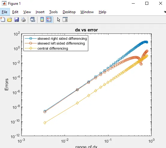
The plot for truncation error for the fourth-order approximation of the second-order derivative for the range of dx. 

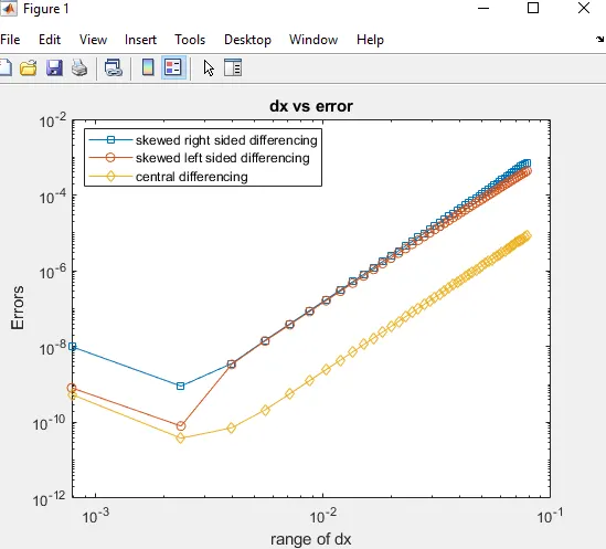
The below plot shows that as the value for dx minimizes after a certain point the error will increases.

 CONCLUSION

Through this challenge, I come to know that

 The central difference gives the lowest error or in other words, we can say that it gives less value of error compared to other schemes.

 The skewed right gives a maximum error as compared to other schemes.

 The skewed left gives error somewhere in between skewed right difference and central difference.

 And also if the range of dx minimizes after a certain point the error also increases that is shown above.

And the plot to compare the fourth-order approximation of the second-order derivative for central difference, skewed-right, and skewed-left difference also plotted.