Week 3 - Solving second order ODEs

OBJECTIVE

• To write the program that solves the second-order ODE which represents the equation of motion of the simple pendulum and damping.
• To create an animation of the motion of the pendulum.

EQUATION USED

`(d^2theta)/(dt^2)+(b/m)*(d(theta))/(dt)+(g/l)sin(theta)=0`

where,

g = gravity in m/s2,

L = length of the pendulum in m,

m = mass of the ball in kg,

b=damping coefficient.

STEPS TO WRITE THE PROGRAM

• Let's start with the clear commands i.e clear all, close all, clc.
• then, defining the inputs by using the comment %inputs i.e b, g, l, m with the given values.
• then, defining the initial conditions i.e theta_0 =[0;3] here 0 is the initial angular displacement and 3m/s is the initial angular velocity, here we are solving the ODE so, we need to provide the initial conditions.
• then we are going to integrating the ODE system to obtain a solution for that we need to define the value for a time by using the comment %time points i.e t_span=linspace(0, 20, 500) here we used the linspace command it says that for the time period of 0 to 20seconds for 500 values in between.
• then we have to call an ODE FUNCTION here it is an anonymous syntax by using the comment %solve ODE i.e [t, results]=ode45(@(t, theta) ode_fun(t, theta, b, g, l, m), t_span, theta_0) here ode45 is an inbuilt solver ode is a function of t, theta.
• will write a function to solve ODE in this case function will be solving the values for theta1 and theta2 actually, here theta1 will be angular displacement and theta2 will be angular displacement. In the function, we are defining the theta1 and theta2 where theta will be the solution array so, the first value theta(1) going to be theta1 and the second value theta(2) Wii going to be theta2.
• then we are defining our first ode i.e dtheta1_dt=theta2 and dtheta_2=-(b/m)*theta2-(g/l)*sin(theta1) and then we separate it as dtheta_dt=[dtheta1_dt; dtheta2_dt] which will be a column matrix. This function will be giving the integration time and the result, since we are solving second-order ODE results will be having two columns first will refer to displacement and the second one will be velocity.
• by using the plot command i.e plot(t, results(:,1)) this will plot the time vs displacement,and plot(t, results(:,2)) will plot the time vs velocity.
• to create an animation we have to create a for loop that should compute for each value of theta so, we are assigning the value i as 1:499 because we are calculating for 500 values so we have given count start as ct=1 and that will be increasing by one count i.e ct=ct+1 so, we are assigning the value how far the iterations to be made.
• then, assigning the x0, y0 as 0 so that it can be considered as the fixing point of the hanging pendulum.
• then, computing the x and y values i.e x1=l*sin(results(i, 1)) and y1=l*(results(i,1)).
• and then creating the mark for the fixed point i.e plot(x0, y0, 'marker', 'square', 'markersize', 25, 'markerfacecolor', 'k').
• Now, creating the mark for the moving point i.e plot(x1, y1, 'marker', 'o', 'markersize', 15, 'markerfacecolor', 'r').
• then, connecting the moving and the fixed point.
• after the end command, we are writing as movie(M) followed by videofile=VideoWriter('pendulum.avi', 'uncompressed AVI'), which will create a video file as pendulum.avi and need to write open(videofile) which will open the file and then to write video need to type writevideo(videofile, M), to close type close(videofile). Then, the animation will be created.

CODE

clear all
close all
clc

%inputs
b=0.05;
g=9.81;
l=1;
m=1;

%initial condition
theta_0=[0;3];

%time points
t_span=linspace(0,20,500);

%solve ODE
[t,results]=ode45(@(t,theta) ode_fun(t,theta,b,g,l,m),t_span,theta_0);

figure(1)
 
plot(t,results(:,1))
hold on
plot(t,results(:,2))

legend('Ang.displacement','Ang.velocity')
xlabel('time (s)')
ylabel('Amplitude')
hold off

 


 




figure(2)

ct=1
for i= 1:499
    x0=0;
    y0=0;
    x1=l*sin(results(i,1));
    y1=-l*cos(results(i,1));
    plot([x0 x1],[y0 y1])
    hold on
    plot(x0,y0,'marker','square','markersize',25,'linewidth',1,'markerfacecolor','k')
 
    plot(x1, y1,'marker','o','markersize',15,'markerfacecolor','r')
    hold off
    axis([-1 1 -1.5 0.5])
    pause(0.03)
    
    M(ct)=getframe(gcf);
    ct=ct+1;
end

movie(M)
videofile=VideoWriter('pendulum.avi','uncompressed AVI');
open(videofile)
writeVideo(videofile,M)
close(videofile)

function [dtheta_dt]=ode_fun(t,theta,b,g,l,m)

dtheta1_dt = theta(2);
dtheta2_dt = -(b/m)*theta(2)-(g/l)*sin(theta(1));
dtheta_dt = [dtheta1_dt; dtheta2_dt];

end

OUTPUT

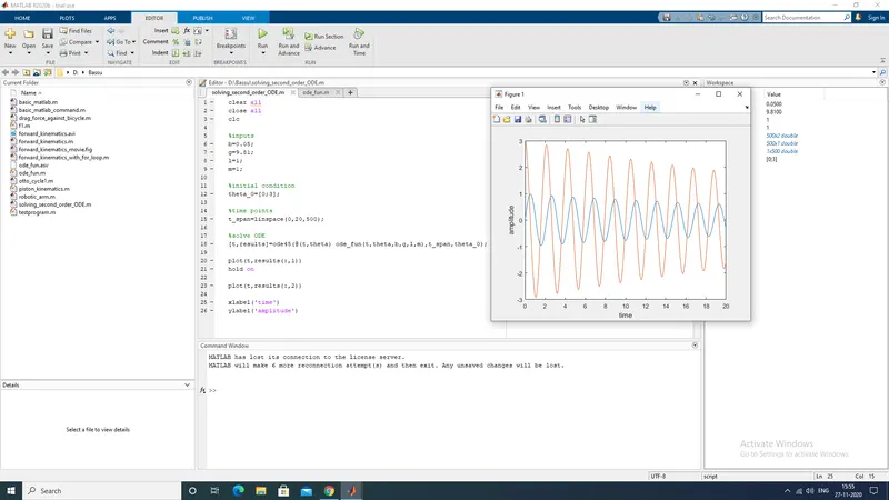
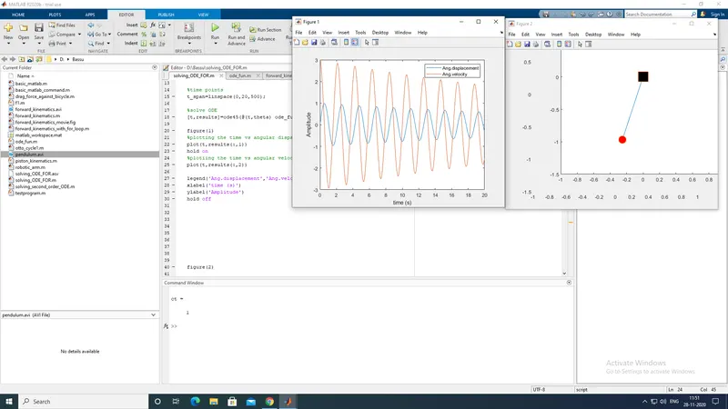
The plot done is as per the given data i.e L=1m, b=0.05, g=9.81, M=1kg, and with the initial condition given are initial displacement as 0 and the initial velocity as 3 rad/s, for the time span of 20 seconds.

ERRORS

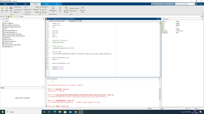
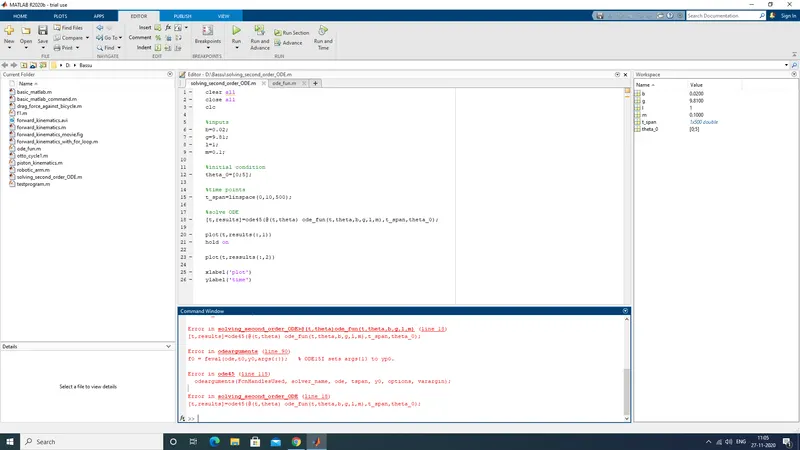
The below error was due to a spelling mistake and it was corrected.

CONCLUSION

Program for simulating the motion of a pendulum and animation for the motion of a pendulum has done.