Week 5 - Mid term project - Solving the steady and unsteady 2D heat conduction problem

Aim: To solve 2D Heat flow equation in steady and transient state conditions using

1.Jacobi method

2.Gauss-Seidel method

3.Successive over relaxation method 

Introduction:

2D heat conduction is studied in this challenge for various methods of iterations.
In real world there is no 2D heat conduction, heat conducts in all 3 dimensions but in this challenge we are neglecting the heat conduction in one dimension to eliminate the complexity in analysing the iterative methods.
The Partial differential equation represnting 2D heat conduction is `(partial T)/(partial t) - alpha*((partial^2 T)/(partial x^2) + (partial^2 T)/(partial y^2) ) = 0`.

 Steady State: State at which there is no change in fluid properties over a period of time is called steady state .Heat conduction at this state is called steady state heat conduction.

Hence for steady state condition

`(partial T)/(partial t)= 0`

`((partial^2 T)/(partial x^2) + (partial^2 T)/(partial y^2) ) = 0`.

Discretizing the equation gives

`(T_L - 2*T_P+T_R)/(Delta x^2) + (T_T - 2*T_P+T_B)/(Delta y^2) = 0`

`k = 2*(Delta x^2 + Deltay^2)/(Deltax^2*Deltay^2)`

For the code

`T_L = T(i-1,j);T_R = T(i+1,j);T_T = T(i,j+1);T_B = T(i,j-1)`

`Deltax =dx;Deltay =dy`

Jacobi Method:

`T^(n+1)=1/K*((T_L+T_R)/(Delta x^2) +(T_B+T_T)/(Delta y^2))^n`

For the code

`k = 2*(dx^2 + dy^2)/(dx^2*dy^2)`

`T(i,j)=(((Told(i-1,j)+Told(i+1,j))/dx^2+(Told(i,j-1)+Told(i,j+1))/dy^2))/k`

Gauss-Seidel Method:

`T^(n+1)=1/K*((T_L+T_R)/(Delta x^2) +(T_B+T_T)/(Delta y^2))^(n+1)`

For the code

`k = 2*(dx^2 + dy^2)/(dx^2*dy^2)`

`T(i,j)=((T(i-1,j)+T(i+1,j))/dx^2+(T(i,j-1)+T(i,j+1))/dy^2)/k`

Successive Over Relaxation:

In SOR we use a factor omega in order to get the convergence sooner but we need to select the omega carefully.

`T^(n+1)=(1-omega)*T^n+omega*(((T_L+T_R)/(Delta x^2) +(T_B+T_T)/(Delta y^2))^(n+1)*1/K)`

For the code

`T(i,j)=(1-omega)*Told(i,j)+omega*(((T(i-1,j)+T(i+1,j))/dx^2+(T(i,j-1)+T(i,j+1))/dy^2)/k)`

Jacobi steady state:

%5.1- Solving 2D heat conduction steady state jacobi 
close all
clear all
clc
%initialization
nx = 10;
ny = nx;
x = linspace(0,1,nx);
y = linspace(0,1,ny);
dx = x(2) - x(1);
dy = y(2) - y(1);
%error limits
error = 9e9;
tol   = 1e-4;
%creating a temperature matrix
T = 300*ones(nx,ny);
%Boundaty conditions (K)
T_Top    = 600; 
T_Bottom = 900; 
T_Left   = 400; 
T_Right  = 800; 
%Assigning values to the temperature matrix
T(1,2:nx-1)  = T_Top;
T(ny,2:nx-1) = T_Bottom;
T(2:ny-1,1)  = T_Left;
T(2:ny-1,nx) = T_Right;
%Approximating corner temperatures
T(1,1)   = (T_Top+T_Left)/2;
T(1,ny)  = (T_Top+T_Right)/2;
T(nx,1)  = (T_Left+T_Bottom)/2;
T(nx,ny) = (T_Right+T_Bottom)/2;

T_old = T;
Tinitial = T;
 
k = 2*(dx^2 + dy^2)/(dx^2*dy^2);

Jacobi_iterative = 1;
Gauss_seidel_iterative = 2;
Successive_over_relaxation_iterative = 3;
%Jacobi_iterative
%  if Jacobi_iterative==1;
tic
    jacobi_iterations = 1;
    while (error > tol)
        for i = 2:nx-1
            for j = 2:ny-1
                T(i,j)=(((T_old(i-1,j)+T_old(i+1,j))/dx^2+(T_old(i,j-1)+T_old(i,j+1))/dy^2))/k;
            end
        end
        error = max(max(abs(T_old-T)));
        jacobi_iterations = jacobi_iterations + 1;
        T_old = T;
        iteration_time = tic
        contourf(x,y,T,'showtext','on');
        colorbar;
        set(gca,'ydir','reverse')
        disp1 = sprintf('No of Jacobi iteratiions = %d',jacobi_iterations);
        disp2 = sprintf('error = %f',error);
        legend('jacobi iterative')
        title(disp1,disp2);
        xlabel('X-axis');
        ylabel('Y-axis');
         pause(0.01);
         pause(0.01);
    end

Gauss Siedel steady state:

%2D heat conduction steady state gauss_seidel
close all
clear all
clc
%initialization
nx = 10;
ny = nx;
x = linspace(0,1,nx);
y = linspace(0,1,ny);
dx = x(2) - x(1);
dy = y(2) - y(1);
%error limits
error = 9e9;
tol   = 1e-4;
%creating a temperature matrix
T = 300*ones(nx,ny);
%Boundaty conditions (K)
T_Top    = 600; 
T_Bottom = 900; 
T_Left   = 400; 
T_Right  = 800; 
%Assigning values to the temperature matrix
T(1,2:nx-1)  = T_Top;
T(ny,2:nx-1) = T_Bottom;
T(2:ny-1,1)  = T_Left;
T(2:ny-1,nx) = T_Right;
%Approximating corner temperatures
T(1,1)   = (T_Top+T_Left)/2;
T(1,ny)  = (T_Top+T_Right)/2;
T(nx,1)  = (T_Left+T_Bottom)/2;
T(nx,ny) = (T_Right+T_Bottom)/2;
%
T_old = T;
Tinitial = T;
 
k = 2*(dx^2 + dy^2)/(dx^2*dy^2);
tic
Gauss_seidel_iterations = 1;
    while (error > tol)
        for i = 2:nx-1
            for j = 2:ny-1
                T(i,j)=((T(i-1,j)+T(i+1,j))/dx^2+(T(i,j-1)+T(i,j+1))/dy^2)/k;
            end
        end
        error = max(max(abs(T_old-T)));
        Gauss_seidel_iterations = Gauss_seidel_iterations + 1;
        T_old = T;
        iteration_time = tic;
        contourf(x,y,T,'showtext','on');
        colorbar;
        colormap;
        set(gca,'ydir','reverse')
        legend('Gauss seidel iterative');
        disp1 = sprintf('No of Gauss seidel iteratiions = %d',Gauss_seidel_iterations);
        disp2 = sprintf('error = %f',error);
        title(disp1,disp2);
        xlabel('X-axis');
        ylabel('Y-axis');
          pause(0.0001);
    end

SOR steady state:

%2D heat conduction steady state SOR 
close all
clear all
clc
%initialization
nx = 10;
ny = nx;
x = linspace(0,1,nx);
y = linspace(0,1,ny);
dx = x(2) - x(1);
dy = y(2) - y(1);
%error limits
error = 9e9;
tol   = 1e-4;
%creating a temperature matrix
T = 300*ones(nx,ny);
%Boundaty conditions (K)
T_Top    = 600; 
T_Bottom = 900; 
T_Left   = 400; 
T_Right  = 800; 
%Assigning values to the temperature matrix
T(1,2:nx-1)  = T_Top;
T(ny,2:nx-1) = T_Bottom;
T(2:ny-1,1)  = T_Left;
T(2:ny-1,nx) = T_Right;
%Approximating corner temperatures
T(1,1)   = (T_Top+T_Left)/2;
T(1,ny)  = (T_Top+T_Right)/2;
T(nx,1)  = (T_Left+T_Bottom)/2;
T(nx,ny) = (T_Right+T_Bottom)/2;

T_old = T;
Tinitial = T;
 
k = 2*(dx^2 + dy^2)/(dx^2*dy^2);
omega=1.2;
%looping
tic
SOR_iterations = 1;
    while (error > tol)
        for i = 2:nx-1
            for j = 2:ny-1
                T(i,j)=(1-omega)*T_old(i,j)+omega*(((T(i-1,j)+T(i+1,j))/dx^2+(T(i,j-1)+T(i,j+1))/dy^2)/k);
            end
        end
        error = max(max(abs(T_old-T)));
        SOR_iterations = SOR_iterations + 1;
        T_old = T;
        iterative_time = toc
        contourf(x,y,T,'showtext','on');
        colorbar;
        set(gca,'ydir','reverse')
        legend('SOR iterative');
        disp1 = sprintf('No of SOR iterations = %d',SOR_iterations);
        disp2 = sprintf('error = %f',error);
        title(disp1,disp2);
        xlabel('X-axis');
        ylabel('Y-axis');
          pause(0.0001);
    end

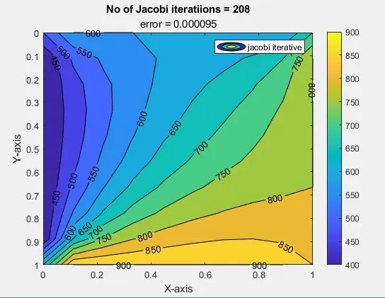
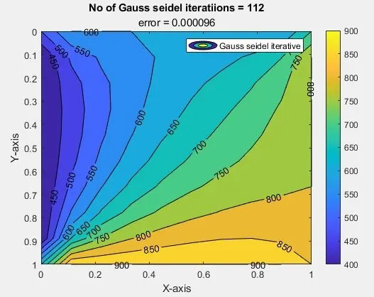
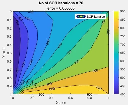
Temperature profile of 2D Steady state heat Conduction :

Jacobi:

Gauss Siedel:

SOR:

Transient State:

• The explicit method and implicit method are numerical analysis methods used to solve a time-dependent differential equation.
• The explicit method calculates the system status at a future time from the currently known system status.
• The implicit method calculates the system status at a future time from the system statuses at present and future times.

Explicit method:

Jacobi :

`k1 = 1.4*(dt/dx^2); k2 = 1.4*(dt/dy^2);`

`T^(n+1) = T_(Initial)^n*(1-(2.K 1) - (2.K 2) ) + (K 1*(T_L^n +T_R^n)) + (K 2*(T_B^n+T_T^n))`

For the code

`k3 = 1-2*k1-2*k2`

`T(i,j) = T(Initial)(i,j)*k3+k1*(Told(i-1,j)+Told(i+1,j))+k2*(Told(i,j+1)+Told(i,j-1))`

Gauss Siedel:

`k1 = 1.4*(dt/dx^2); k2 = 1.4*(dt/dy^2);

`T^(n+1) = T_(Initial)^n*(1-(2.K 1) - (2.K 2) ) + (K 1*(T_L^(n+1) +T_R^n)) + (K 2*(T_T^n+T_B^(n+1)))`

For the code

`k3 = 1-2*k1-2*k2`

`T(i,j) = T(Initial)(i,j)*k3+k1*(T(i-1,j)+Told(i+1,j))+k2*(Told(i,j+1)+T(i,j-1));`

Successive Over Relaxation:

`T^(n+1) = T_(Initial)^n*(1-omega) + omega*[T_(Initial)^n*(1-(2.K 1) - (2.K 2) ) + (K 1*(T_L^(n+1) +T_R^n)) + (K 2*(T_T^n+T_B^(n+1)))]`

For the code

`k3 = 1-2*k1-2*k2`

`T(i,j) = (1-omega)*Told(i,j)+omega*(T(Initial)(i,j)*k3+k1*(T(i-1,j)+Told(i+1,j))+k2*(Told(i,j+1)+T(i,j-1)));`

Matlab Code for Explicit Jacobi:

%2D heat conduction jacobi Explicit
close all
clear all
clc
%initialization
nx = 10;
ny = nx;
nt = 1400;
x = linspace(0,1,nx);
y = linspace(0,1,ny);
dx = x(2) - x(1);
dy = dx;
dt = 1e-3;
omega = 1.1;
%error limits
error = 9e9;
tol   = 1e-4;
%creating a temperature matrix
T = 300*ones(nx,ny);
%Boundaty conditions (K)
T_Top    = 600; 
T_Bottom = 900; 
T_Left   = 400; 
T_Right  = 800; 
%Assigning values to the temperature matrix
T(1,2:nx-1)  = T_Top;
T(ny,2:nx-1) = T_Bottom;
T(2:ny-1,1)  = T_Left;
T(2:ny-1,nx) = T_Right;
%Approximating corner temperatures
T(1,1)   = (T_Top+T_Left)/2;
T(1,ny)  = (T_Top+T_Right)/2;
T(nx,1)  = (T_Left+T_Bottom)/2;
T(nx,ny) = (T_Right+T_Bottom)/2;

T_old = T;
Tinitial = T;
k1 = 1.4*(dt/dx^2);
k2 = 1.4*(dt/dy^2);
 k3 = 1-2*k1-2*k2
CFL = k1 +k2
alpha=1.2;
%looping
jacobi_iterations = 1;
for k =1:nt
    error = 9e9;
    while (error > tol)
        for i = 2:nx-1
            for j = 2:ny-1
                T(i,j) = Tinitial(i,j)*k3+k1*(T_old(i-1,j)+T_old(i+1,j))+k2*(T_old(i,j+1)+T_old(i,j-1));
                
            end
        end
        error = max(max(abs(T_old-T)));
        T_old = T;
        jacobi_iterations = jacobi_iterations + 1;
      
    end
        Tinitial = T;
        contourf(x,y,T,'showtext','on');
        colorbar;
        colormap(winter);
        set(gca,'ydir','reverse')
        legend('jacobi Explicit');
        disp1 = sprintf('No of jacobi(Explicit)iterations = %d',jacobi_iterations);
        title(disp1);
        xlabel('X-axis');
        ylabel('Y-axis');
          pause(0.0001);
end

   

Matlab Code for Explicit Gauss Siedel:

%2D heat conduction gauss seidel Explicit
close all
clear all
clc
%initialization
nx = 10;
ny = nx;
nt = 1400;
x = linspace(0,1,nx);
y = linspace(0,1,ny);
dx = x(2) - x(1);
dy = dx;
dt = 1e-3;
omega = 1.1;
%error limits
error = 9e9;
tol   = 1e-4;
%creating a temperature matrix
T = 300*ones(nx,ny);
%Boundaty conditions (K)
T_Top    = 600; 
T_Bottom = 900; 
T_Left   = 400; 
T_Right  = 800; 
%Assigning values to the temperature matrix
T(1,2:nx-1)  = T_Top;
T(ny,2:nx-1) = T_Bottom;
T(2:ny-1,1)  = T_Left;
T(2:ny-1,nx) = T_Right;
%Approximating corner temperatures
T(1,1)   = (T_Top+T_Left)/2;
T(1,ny)  = (T_Top+T_Right)/2;
T(nx,1)  = (T_Left+T_Bottom)/2;
T(nx,ny) = (T_Right+T_Bottom)/2;

T_old = T;
Tinitial = T;
k1 = 1.4*(dt/dx^2);
k2 = 1.4*(dt/dy^2);
k3 = 1-2*k1-2*k2;
alpha=1.2;
%looping
G_S_iterations = 1;
for k =1:nt
    error = 9e9;
    while (error > tol)
        for i = 2:nx-1
            for j = 2:ny-1
                T(i,j) = Tinitial(i,j)*k3+k1*(T(i-1,j)+T_old(i+1,j))+k2*(T_old(i,j+1)+T(i,j-1));
                
            end
        end
        error = max(max(abs(T_old-T)));
        T_old = T;
        G_S_iterations = G_S_iterations + 1;
      
    end
        Tinitial = T;
        contourf(x,y,T,'showtext','on');
        colorbar;
        colormap(winter);
        set(gca,'ydir','reverse')
        legend('Gauss seidel Explicit');
        disp1 = sprintf('No of Gauss seidel(Explicit)iterations = %d',G_S_iterations);
        title(disp1);
        xlabel('X-axis');
        ylabel('Y-axis');
          pause(0.0001);
    end

Matlab Code for Explicit SOR:

%2D heat conduction SOR Explicit
close all
clear all
clc
%initialization
nx = 10;
ny = nx;
nt = 1400;
x = linspace(0,1,nx);
y = linspace(0,1,ny);
dx = x(2) - x(1);
dy = dx;
dt = 1e-3;
omega = 1.1;
%error limits
error = 9e9;
tol   = 1e-4;
%creating a temperature matrix
T = 300*ones(nx,ny);
%Boundaty conditions (K)
T_Top    = 600; 
T_Bottom = 900; 
T_Left   = 400; 
T_Right  = 800; 
%Assigning values to the temperature matrix
T(1,2:nx-1)  = T_Top;
T(ny,2:nx-1) = T_Bottom;
T(2:ny-1,1)  = T_Left;
T(2:ny-1,nx) = T_Right;
%Approximating corner temperatures
T(1,1)   = (T_Top+T_Left)/2;
T(1,ny)  = (T_Top+T_Right)/2;
T(nx,1)  = (T_Left+T_Bottom)/2;
T(nx,ny) = (T_Right+T_Bottom)/2;

T_old = T;
Tinitial = T;
k1 = 1.4*(dt/dx^2);
k2 = 1.4*(dt/dy^2);
k3 = 1-2*k1-2*k2;
alpha=1.2;
%looping
SOR_iterations = 1;
for k =1:nt
    error = 9e9;
    while (error > tol)
        for i = 2:nx-1
            for j = 2:ny-1
                T(i,j) = (1-omega)*T_old(i,j)+omega*(Tinitial(i,j)*k3+k1*(T(i-1,j)+T_old(i+1,j))+k2*(T_old(i,j+1)+T(i,j-1)));
                
            end
        end
        error = max(max(abs(T_old-T)));
        T_old = T;
        SOR_iterations = SOR_iterations + 1;
      
    end
        Tinitial = T;
        contourf(x,y,T,'showtext','on');
        colorbar;
        colormap(winter);
        set(gca,'ydir','reverse')
        legend('SOR Explicit');
        disp1 = sprintf('No of SOR(Explicit)iterations = %d',SOR_iterations);
        title(disp1);
        xlabel('X-axis');
        ylabel('Y-axis');
          pause(0.0001);
 end
    

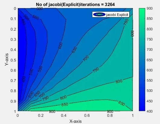
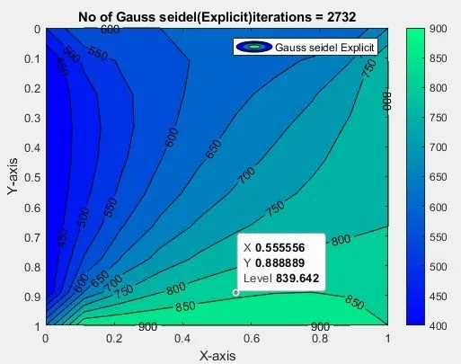
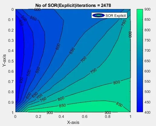
Temperature profile of 2D Transient heat Conduction(Explicit) :

Jacobi :

Gauss Siedel:

SOR:

Implicit Method:

Jacobi :

`T^(n+1) = (T_(Initial)^n + K 1*(T_L^(n)+ T_R^n) + K 2*(T_T^(n) + T_B^n) ) / (1+2*K 1+2*K 2)`

For the code

`k1 = 1.4*(dt/dx^2); k2 = 1.4*(dt/dy^2);`

`den = 1+2*k1+2*k2`

`Num = TInitial(i,j)+k1*(Told(i-1,j)+Told(i+1,j))+k2*(Told(i,j+1)+Told(i,j-1)); T(i,j)=(Num)/(den);`

Gauss Siedel:

`T^(n+1) = (T_(Initial)^n + K 1*(T_L^(n+1)+ T_R^(n)) + K 2*(T_T^(n) + T_B^(n+1)) ) / (1+2*K 1+2*K 2)`

for the code

`k1 = 1.4*(dt/dx^2); k2 = 1.4*(dt/dy^2);`

`den = 1+2*k1+2*k2`

`Num = TInitial(i,j)+k1*(T(i-1,j)+Told(i+1,j))+k2*(Told(i,j+1)+T(i,j-1)); T(i,j)=(Num)/(den)`

SOR:

`T^(n+1) = T_(Initial)^n*(1-omega) + omega*[(T_(Initial)^n + K 1*(T_L^(n+1)+ T_R^(n)) + K 2*(T_T^(n) + T_B^(n+1)) ) / (1+2*K 1+2*K 2)]`

`den = 1+2*k1+2*k2`

`Num = TInitial(i,j)+k1*(T(i-1,j)+Told(i+1,j))+k2*(Told(i,j+1)+T(i,j-1)); T(i,j)=(1-omega)*Told(i,j)+omega*((Num)/(den))`

Matlab Code for Implicit Jacobi:

%2D heat conduction steady state jacobi Implicit
close all
clear all
clc
%initialization
nx = 10;
ny = nx;
nt = 1400;
x = linspace(0,1,nx);
y = linspace(0,1,ny);
dx = x(2) - x(1);
dy = dx;
dt = 1e-3;
omega = 1.1;
%error limits
error = 9e9;
tol   = 1e-4;
%creating a temperature matrix
T = 300*ones(nx,ny);
%Boundaty conditions (K)
T_Top    = 600; 
T_Bottom = 900; 
T_Left   = 400; 
T_Right  = 800; 
%Assigning values to the temperature matrix
T(1,2:nx-1)  = T_Top;
T(ny,2:nx-1) = T_Bottom;
T(2:ny-1,1)  = T_Left;
T(2:ny-1,nx) = T_Right;
%Approximating corner temperatures
T(1,1)   = (T_Top+T_Left)/2;
T(1,ny)  = (T_Top+T_Right)/2;
T(nx,1)  = (T_Left+T_Bottom)/2;
T(nx,ny) = (T_Right+T_Bottom)/2;

T_old = T;
Tinitial = T;
k1 = 1.4*(dt/dx^2);
k2 = 1.4*(dt/dy^2);

den = 1+2*k1+2*k2;
alpha=1.4;
%looping
jacobi_iterations = 1;
for k =1:nt
    error = 9e9;
    while (error > tol)
        for i = 2:nx-1
            for j = 2:ny-1
                num = Tinitial(i,j)+k1*(T_old(i-1,j)+T_old(i+1,j))+k2*(T_old(i,j+1)+T_old(i,j-1));
                T(i,j)=num/den;
            end
        end
        error = max(max(abs(T_old-T)));
        T_old = T;
        jacobi_iterations = jacobi_iterations + 1;
      
    end
        Tinitial = T;
        contourf(x,y,T,'showtext','on');
        colorbar;
        colormap(jet);
        set(gca,'ydir','reverse')
        legend('jacobi Implicit');
        disp1 = sprintf('No of jacobi(Implicit)iterations = %d',jacobi_iterations);
        title(disp1);
        xlabel('X-axis');
        ylabel('Y-axis');
          pause(0.0001);
    end

Matlab Code for Implicit Gauss Siedel:

%2D heat conduction Gauss seidel Implicit
close all
clear all
clc
%initialization
nx = 10;
ny = nx;
nt = 1400;
x = linspace(0,1,nx);
y = linspace(0,1,ny);
dx = x(2) - x(1);
dy = dx;
dt = 1e-3;
omega = 1.1;
%error limits
error = 9e9;
tol   = 1e-4;
%creating a temperature matrix
T = 300*ones(nx,ny);
%Boundaty conditions (K)
T_Top    = 600; 
T_Bottom = 900; 
T_Left   = 400; 
T_Right  = 800; 
%Assigning values to the temperature matrix
T(1,2:nx-1)  = T_Top;
T(ny,2:nx-1) = T_Bottom;
T(2:ny-1,1)  = T_Left;
T(2:ny-1,nx) = T_Right;
%Approximating corner temperatures
T(1,1)   = (T_Top+T_Left)/2;
T(1,ny)  = (T_Top+T_Right)/2;
T(nx,1)  = (T_Left+T_Bottom)/2;
T(nx,ny) = (T_Right+T_Bottom)/2;

T_old = T;
Tinitial = T;
k1 = 1.4*(dt/dx^2);
k2 = 1.4*(dt/dy^2);

den = 1+2*k1+2*k2;
alpha=1.2;
%looping
G_s_iterations = 1;
for k =1:nt
    error = 9e9;
    while (error > tol)
        for i = 2:nx-1
            for j = 2:ny-1
                num = Tinitial(i,j)+k1*(T(i-1,j)+T_old(i+1,j))+k2*(T_old(i,j+1)+T(i,j-1));
                T(i,j)=num/den;
            end
        end
        error = max(max(abs(T_old-T)));
        T_old = T;
        G_s_iterations = G_s_iterations + 1;
      
    end
        Tinitial = T;
        contourf(x,y,T,'showtext','on');
        colorbar;
        colormap(jet);
        set(gca,'ydir','reverse')
        legend('Gauss seidel Implicit');
        disp1 = sprintf('No of Gauss seidel(Implicit)iterations = %d',G_s_iterations);
        disp2 = sprintf('error = %f',error);
        title(disp1,disp2);
        xlabel('X-axis');
        ylabel('Y-axis');
          pause(0.03);
    end

Matlab Code for Implicit SOR:

%2D heat conduction SOR Implicit
close all
clear all
clc
%initialization
nx = 10;
ny = nx;
x = linspace(0,1,nx);
y = linspace(0,1,ny);
dx = x(2) - x(1);
dy = y(2) - y(1);
dt = 1e-3;
omega = 1.1;
%error limits
error = 9e9;
tol   = 1e-4;
%creating a temperature matrix
T = 300*ones(nx,ny);
%Boundaty conditions (K)
T_Top    = 600; 
T_Bottom = 900; 
T_Left   = 400; 
T_Right  = 800; 
%Assigning values to the temperature matrix
T(1,2:nx-1)  = T_Top;
T(ny,2:nx-1) = T_Bottom;
T(2:ny-1,1)  = T_Left;
T(2:ny-1,nx) = T_Right;
%Approximating corner temperatures
T(1,1)   = (T_Top+T_Left)/2;
T(1,ny)  = (T_Top+T_Right)/2;
T(nx,1)  = (T_Left+T_Bottom)/2;
T(nx,ny) = (T_Right+T_Bottom)/2;

T_old = T;
Tinitial = T;
nt = 1400; 
k1 = 1.4*(dt/dx^2);
k2 = 1.4*(dt/dy^2);

den = 1+2*k1+2*k2;
alpha=1.2;
%looping
SOR_iterations = 1;
for k =1:nt
    error = 9e9;
    while (error > tol)
        for i = 2:nx-1
            for j = 2:ny-1
                num = Tinitial(i,j)+k1*(T(i-1,j)+T_old(i+1,j))+k2*(T_old(i,j+1)+T(i,j-1));
                T(i,j)=(1-omega)*T_old(i,j)+omega*(num/den);
            end
        end
        error = max(max(abs(T_old-T)));
        T_old = T;
        SOR_iterations = SOR_iterations + 1;
      
    end
        Tinitial = T;
        contourf(x,y,T,'showtext','on');
        colorbar;
        colormap(jet);
        set(gca,'ydir','reverse')
        legend('SOR Implicit');
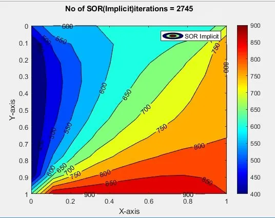
        disp1 = sprintf('No of SOR(Implicit)iterations = %d',SOR_iterations);
        title(disp1);
        xlabel('X-axis');
        ylabel('Y-axis');
          pause(0.03);
    end

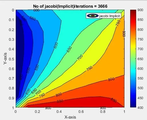
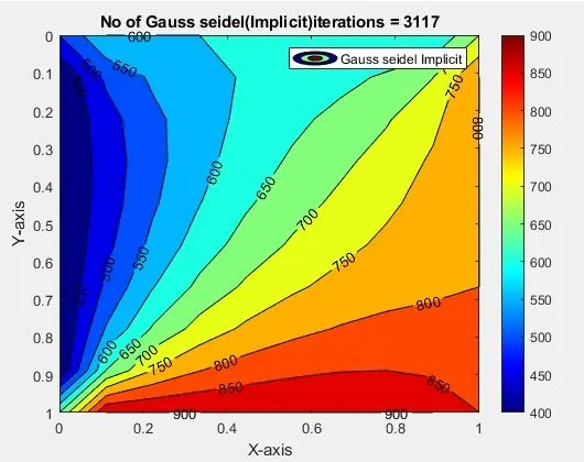
Temperature profile of 2D Transient heat Conduction(Implicit) :

Jacobi:

Gauss Siedel:

SOR:

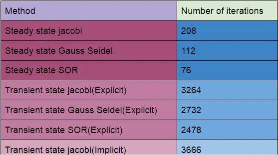
Number of iterations For each method:

Conclusion from the Temperature Profiles:

• Steady state methods results in the faster convergence which means less number of iterations.
• Transient state methods take longer duration to converge or take higher number of iterations.
• Comparing jacobi,Gauss Siedel and Successive Over Relaxation we can see from the plots that Successive Over Relaxation gives results in least iterations.
• Highest number of Iterations are seen in the Jacobi Schemes .