Week 5 - Mid term project - Solving the steady and unsteady 2D heat conduction problem
AIM: To solve the 2D heat conduction equation by using the point iterative techniques namely Jacobi, Gauss Siedel and Successive over relaxation methods for steady state and transient analysis.
Method: For steady state:
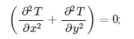
The heat conduction equation that needs to be solved is:
Discretizing the above equation with respect to central difference scheme gives:
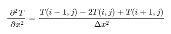
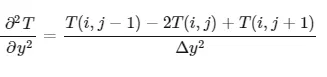
Substituting the values into the steady state heat condunction equation, it follows that:

The MATLAB codes for solving the equation through all the iterative methods is given below:
clear all
close all
clc
% Using jacobi iterations


l=1; % defining the length of the domain
nx=30; % number of discritizing units in horizontal direction
ny=nx;
x=linspace(0,l,nx); %dividing the domain into equal number of units
y=linspace(0,l,ny);
dx=x(2)-x(1); %length of each discretizing unit
dy=y(2)-y(1);
err=9e9
tol=1e-4 %defining the tolerance

%boundary conditions
Tl=400;
Tt=600;
Tr=800;
Tb=900;
T=ones(nx,ny)
% Assigning the temperature values at all four edges of the domain.
T(2:ny-1,1)=Tl;
T(2:ny-1,nx)=Tr;
T(1,2:nx-1)=Tt;
T(nx,2:ny-1)=Tb;

%Calculating average temperture at the four corners

T(1,1)=(Tl+Tt)/2;
T(1,ny)=(Tt+Tr)/2;
T(nx,1)=(Tl+Tb)/2;
T(nx,ny)=(Tr+Tb)/2;

%creating a mesh grid of the values
[X,Y]=meshgrid(x,y);
Told=T;

% finding the temperature profile through Jacobi iterations
tic

jacobi_iter=1;
while(err>tol)
    for i=2:nx-1
        for j=2:ny-1
            T(i,j)=0.25*((Told(i-1,j)+Told(i+1,j)+Told(i,j-1)+Told(i,j+1)));
        end
    end
    err=max(max((abs(Told-T))));
    Told=T;
    jacobi_iter=jacobi_iter+1;
end
F=toc;
% plotting the final figure
    figure(1)
    [M,N]=contourf(X,Y,T);
    clabel(M,N);
    text=sprintf('Total time passed= %fs',F);
    title(text)
    colorbar
    xlabel('X-axis')
    ylabel('Y-axis')
    fprintf('Total number of iterations in Jacobi for stable solution=%d\n',jacobi_iter);
clear all
close all
clc
% Using gauss siedel method


l=1; % defining the length of the domain
nx=30; % number of discritizing units in horizontal direction
ny=nx;
x=linspace(0,l,nx); %dividing the domain into equal number of units
y=linspace(0,l,ny);
dx=x(2)-x(1); %length of each discretizing unit
dy=y(2)-y(1);
err=9e9
tol=1e-4 %defining the tolerance

%boundary conditions
Tl=400;
Tt=600;
Tr=800;
Tb=900;
T=ones(nx,ny)
% Assigning the temperature values at all four edges of the domain.
T(2:ny-1,1)=Tl;
T(2:ny-1,nx)=Tr;
T(1,2:nx-1)=Tt;
T(nx,2:ny-1)=Tb;

%Calculating average temperture at the four corners

T(1,1)=(Tl+Tt)/2;
T(1,ny)=(Tt+Tr)/2;
T(nx,1)=(Tl+Tb)/2;
T(nx,ny)=(Tr+Tb)/2;

%creating a mesh grid of the values
[X,Y]=meshgrid(x,y);
Told=T;

% finding the temperature profile through Jacobi iterations
tic

gs_iter=1;
while(err>tol)
    for i=2:nx-1
        for j=2:ny-1
            T(i,j)=0.25*((T(i-1,j)+Told(i+1,j)+T(i,j-1)+Told(i,j+1)));
        end
    end
    err=max(max((abs(Told-T))));
    Told=T;
    gs_iter=gs_iter+1;
end
F=toc;
% plotting the final figure
    figure(1)
    [M,N]=contourf(X,Y,T);
    clabel(M,N);
    text=sprintf('Total time passed= %fs',F);
    title(text)
    colorbar
    xlabel('X-axis')
    ylabel('Y-axis')
    fprintf('Total number of iterations in gasuss siedel for stable solution=%d\n',gs_iter);
clear all
close all
clc
% Using successive over relaxation method


l=1; % defining the length of the domain
nx=30; % number of discritizing units in horizontal direction
ny=nx;
x=linspace(0,l,nx); %dividing the domain into equal number of units
y=linspace(0,l,ny);
dx=x(2)-x(1); %length of each discretizing unit
dy=y(2)-y(1);
err=9e9
tol=1e-4 %defining the tolerance

%boundary conditions
Tl=400;
Tt=600;
Tr=800;
Tb=900;
T=ones(nx,ny)
% Assigning the temperature values at all four edges of the domain.
T(2:ny-1,1)=Tl;
T(2:ny-1,nx)=Tr;
T(1,2:nx-1)=Tt;
T(nx,2:ny-1)=Tb;

%Calculating average temperture at the four corners

T(1,1)=(Tl+Tt)/2;
T(1,ny)=(Tt+Tr)/2;
T(nx,1)=(Tl+Tb)/2;
T(nx,ny)=(Tr+Tb)/2;

%creating a mesh grid of the values
[X,Y]=meshgrid(x,y);
Told=T;

%defining the alpha parameter
a=1.8
% finding the temperature profile through SOR
tic

sor_iter=1;
while(err>tol)
    for i=2:nx-1
        for j=2:ny-1
            T(i,j)=((1-a)*Told(i,j)+(a*0.25*(T(i,j-1)+Told(i,j+1)+T(i-1,j)+Told(i+1,j))));
        end
    end
    err=max(max((abs(Told-T))));
    Told=T;
    sor_iter=sor_iter+1;
end
F=toc;
% plotting the final figure
    figure(1)
    [M,N]=contourf(X,Y,T);
    clabel(M,N);
    text=sprintf('Total time passed= %fs',F);
    title(text)
    colorbar
    xlabel('X-axis')
    ylabel('Y-axis')
    fprintf('Total number of iterations in SOR for stable solution=%d\n',sor_iter);
Results and plots for steady state:
Plot obtained through Jacobi method:
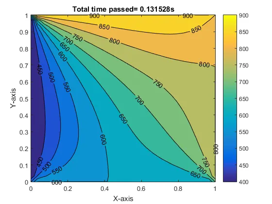
Plot obtained through Gauss siedel method:
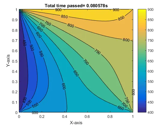
Plot obtained through SOR method:
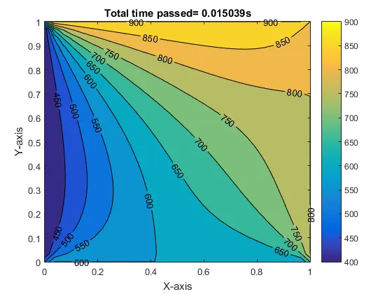
Transient state analysis:
The 2D heat conduction equation is for transient state is given as:
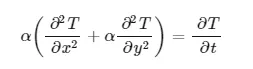
The solution can be found both implicitly and explicitly using the three iterative methods.
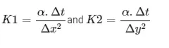
Discretization of the equation gives:

Here
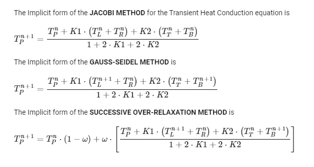
The implicit method code for Jacobi (Transient):
clear all
close all
clc
%Solving the transient equation

l=1; % defining the length of the domain
nx=10; % number of discritizing units in horizontal direction
ny=nx;
x=linspace(0,l,nx); %dividing the domain into equal number of units
y=linspace(0,l,ny);
dx=x(2)-x(1); %length of each discretizing unit
dy=y(2)-y(1);
err=9e9
tol=1e-4;%defining the tolerance

dt=1e-3; % time step

% thermal diffusivity for steel
a=1.9e-5

%boundary conditions
Tl=400;
Tt=600;
Tr=800;
Tb=900;
T=ones(nx,ny)
% Assigning the temperature values at all four edges of the domain.
T(2:ny-1,1)=Tl;
T(2:ny-1,nx)=Tr;
T(1,2:nx-1)=Tt;
T(nx,2:ny-1)=Tb;

%Calculating average temperture at the four corners

T(1,1)=(Tl+Tt)/2;
T(1,ny)=(Tt+Tr)/2;
T(nx,1)=(Tl+Tb)/2;
T(nx,ny)=(Tr+Tb)/2;

% calculation of constants
k1=(1.1*dt)/(dx^2);
k2=(1.1*dt)/(dy^2);

%creating a mesh grid of the values
%[X,Y]=meshgrid(x,y);
Told=T;
T_init=T
% finding the temperature profile through explicit method

jacobi_iter=1
nt=1400
for m=1:nt
    err=9e9;

    while(err>tol)
        for i=2:(nx-1)

            for j=2:(ny-1)
                t1=1/(1+(2*k1)+(2*k2));
                t2=k1*t1
                t3=k2*t1
                H=Told(i-1,j)+Told(i+1,j);
                V=Told(i,j+1)+Told(i,j-1);
                T(i,j)=(T_init(i,j)*t1)+(H*t2)+(V*t3);
            end
        end
        err=max(max(abs(Told-T)));
        Told=T;
        jacobi_iter= jacobi_iter+1;
    end
    T_init=T

    figure(1)
    [M,N]=contourf(x,y,T);
    clabel(M,N);

    colorbar
    xlabel('X-axis')
    ylabel('Y-axis')
    fprintf('Total number of iterations in Jacobi for stable solution=%d\n',jacobi_iter);
    pause(0.01)

end
The implicit code for Gauss Siedel Method(Transient):
clear all
close all
clc
%Solving the transient equation

l=1; % defining the length of the domain
nx=10; % number of discritizing units in horizontal direction
ny=nx;
x=linspace(0,l,nx); %dividing the domain into equal number of units
y=linspace(0,l,ny);
dx=x(2)-x(1); %length of each discretizing unit
dy=y(2)-y(1);
err=9e9
tol=1e-4;%defining the tolerance

dt=1e-3; % time step

% thermal diffusivity for steel
a=1.9e-5

%boundary conditions
Tl=400;
Tt=600;
Tr=800;
Tb=900;
T=ones(nx,ny)
% Assigning the temperature values at all four edges of the domain.
T(2:ny-1,1)=Tl;
T(2:ny-1,nx)=Tr;
T(1,2:nx-1)=Tt;
T(nx,2:ny-1)=Tb;

%Calculating average temperture at the four corners

T(1,1)=(Tl+Tt)/2;
T(1,ny)=(Tt+Tr)/2;
T(nx,1)=(Tl+Tb)/2;
T(nx,ny)=(Tr+Tb)/2;

% calculation of constants
k1=(1.1*dt)/(dx^2);
k2=(1.1*dt)/(dy^2);

%creating a mesh grid of the values
%[X,Y]=meshgrid(x,y);
Told=T;
T_init=T
% finding the temperature profile through explicit method

GS_iter=1
nt=1400
for m=1:nt
    err=9e9;

    while(err>tol)
        for i=2:(nx-1)

            for j=2:(ny-1)
                t1=1/(1+(2*k1)+(2*k2));
                t2=k1*t1
                t3=k2*t1
                H=Told(i-1,j)+Told(i+1,j);
                V=Told(i,j+1)+Told(i,j-1);
                T(i,j)=(T_init(i,j)*t1)+(H*t2)+(V*t3);
            end
        end
        err=max(max(abs(Told-T)));
        Told=T;
        GS_iter= GS_iter+1;
    end
    T_init=T

    figure(1)
    [M,N]=contourf(x,y,T);
    clabel(M,N);

    colorbar
    xlabel('X-axis')
    ylabel('Y-axis')
    fprintf('Total number of iterations in GS for stable solution=%d\n',GS_iter);
    pause(0.01)

end
Implicit method, Successive over Relaxation(SOR):
clear all
close all
clc
%Solving the transient equation

l=1; % defining the length of the domain
nx=10; % number of discritizing units in horizontal direction
ny=nx;
x=linspace(0,l,nx); %dividing the domain into equal number of units
y=linspace(0,l,ny);
dx=x(2)- x(1); %length of each discretizing unit
dy=y(2)- y(1);
err=9e9
tol=1e-4;%defining the tolerance

dt=1e-3; % time step

% thermal diffusivity for steel
a=1.9e-5

%boundary conditions
Tl=400;
Tt=600;
Tr=800;
Tb=900;
T=ones(nx,ny)
% Assigning the temperature values at all four edges of the domain.
T(2:ny-1,1)=Tl;
T(2:ny-1,nx)=Tr;
T(1,2:nx-1)=Tt;
T(nx,2:ny-1)=Tb;

%Calculating average temperture at the four corners

T(1,1)=(Tl+Tt)/2;
T(1,ny)=(Tt+Tr)/2;
T(nx,1)=(Tl+Tb)/2;
T(nx,ny)=(Tr+Tb)/2;

% calculation of constants
k1=(1.1*dt)/(dx^2);
k2=(1.1*dt)/(dy^2);

%creating a mesh grid of the values
%[X,Y]=meshgrid(x,y);
Told=T;
T_init=T;
Tend=T;
omega=1.1
% finding the temperature profile through explicit method

SOR_iter=1
nt=1400
for m=1:nt
    err=9e9;

    while(err>tol)
        for i=2:(nx-1)

            for j=2:(ny-1)
                t1=1/(1+(2*k1)+(2*k2));
                t2=k1*t1
                t3=k2*t1
                H=Told(i-1,j)+Told(i+1,j);
                V=Told(i,j+1)+Told(i,j-1);
                T(i,j)=(T_init(i,j)*t1)+(H*t2)+(V*t3);
                Tend(i,j)=((1-omega)*Told(i,j))+(T(i,j)*omega);
            end
        end
        err=max(max(abs(Told-T)));
        Told=Tend;
        SOR_iter= SOR_iter+1;
    end
    T_init=T

    figure(1)
    [M,N]=contourf(x,y,T);
    clabel(M,N);

    colorbar
    xlabel('X-axis')
    ylabel('Y-axis')
    fprintf('Total number of iterations in SOR for stable solution=%d\n',SOR_iter);
    pause(0.01)

end
The time varying temperature profile animation video link for SOR method is given:
https://drive.google.com/file/d/19yPSu-3ePFUzzXXBuSJVSAasc4urGSwb/view?usp=sharing
CONCLUSIONS: From the results generated for all the iterative methods, it follows that the number of iterations for Jacobi > Gauss Siedel> Successive over relaxation. The most effective method in this case would be SOR since the number of iterations for converging solution is much less than the other two.