Week 5 - Mid term project - Solving the steady and unsteady 2D heat conduction problem

TITLE :

Solving the steady and unsteady two dimensional heat conduction problem.

THEORY:

The generalised heat conduction equation equation with or without heat generation:

`(del^2T)/(delx^2)+(del^2T)/(dely^2)+(del^2T)/(delz^2)+q/k=1/alpha*(delT)/(delt)` ---(1)

where,

T denotes temperature.

q denotes the heat generation inside the body .

k denotes the thermal conductivity of the material.

`alpha`denotes the thermal diffusivity .

Now, if the heat generation within the body is assumed to be zero , then the generalised heat conduction equation reduces to :

`(del^2T)/(delx^2) + (del^2T)/(dely^2) +(del^2T)/(delz^2) = 1/alpha*(delT)/(delt)`---(2)

equation (2) is the unsteady state heat conduction equation.

For the equation to be steady state , the right hand side of the equation (2) have to be zero

Considering only the two dimensional state ;

`(del^2T)/(delx^2)+(del^2T)/(dely^2) = 0`----(3)

equation (3) is the two dimensional steady state heat conduction equation.

DISCRETIZATION :

The steady state equation is discretized and that is solved at all the nodes.

The space derivatives are discretized using the second order cenral second differencing scheme :

`(T(i+1,j) - 2*T(i,j) +T(i-1,j))/(deltax)^2 +(T(i,j+1)-2*T(i,j)+T(i,j-1))/(deltay)^2 = 0`---(4)

In the above equation, `T(i,j)`is the point under consideration. (i+1) is the node at the right , (i-1) is the node at the left. (j+1) is the node at the top and (j-1) is the node at the bottom.

So , this is a elleptical space we are considering.

PROBLEM DESCRIPTION:

Top Boundary = 600 K

Bottom Boundary = 900 K

Left Boundary = 400 K

Right Boundary = 800 K

The temperatures at the wall are provided. The edge temparatures are calculated from the above data.

The steady state and the transient heat conduction problem should be solved using the point iterative techniques like Gauss siedel, Jacabi iterative method and SOR method.

MATLAB MODELLING:

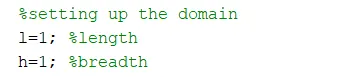
• To set up the domain, the dimensions of the space are provided. The length of that domain is 1 units and breadth is 1 units .

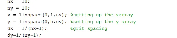
• The x and y array is generated using the linspace command . nx and ny values are provided. Since `deltax = deltay`, so nx = ny . dx and dy are the grit spacing. Uniform grit spacing is chosen.

• The initial temperature inside the domain at all the nodes is guessed as 350K , the boundary temperatures are provided in the problem citation. This is the initial guess. To create a matrix , we provide the command 350*ones(nx,ny) . This looks like this:

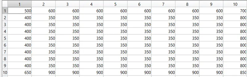
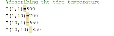
• This is a 10*10 matrix . The edge temperatures are calculated by averaging . for example , Temperature at first row and irst column is the average of the temperature beteen first row second column and second row first column. Similarly all other edge temperatures are calculated.

• A 2D array is formed using the command meshgrid. The inputs are the x and the y values. The tolerance and the error values are provided.

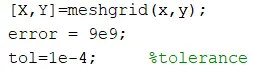
• The problem is solved using the iterative technique. The current node under consideration needs to be updated with values of the previous node. thats why T_old = T , since dx=dy , nx=ny , so the k value is also updated.

• In this problem we use three iterative solvers, namely Jacobi, gauss siedel and SOR. The corresponding serial number is chosen using a if loop, then the logic is , while the error is greater than tolerance value , amd looping through the x axis nodes and the y axis nodes, We calculate the T(i,j) values for the diferent iterative techniques. The time for simulatin and the number of iterations is calculated and displayed.
• Three separate figure windows are created to plot the resiukts obtained for three different cases. contour plot is created using the command contourf.

MATLAB CODE:

%steady state analysis
%Setting up the domain
l = 1; %length
h=1;   %breadth
nx=10; %number of nodes
ny = 10;
x = linspace(0,l,nx); %creating the x array
y = linspace(0,h,ny);  %creating the y array
dx = 1/(nx-1);        %grit spacing
dy=1/(ny-1);

%setting the temperature profile
T=350*ones(nx,ny); %initial guess temperature
T(:,1)=400;        %boundary temprature(left)
T(:,nx)=800;       %boundary temperature(right)
T(1,:)=600;        %boundary temperature(top)
T(ny,:)=900;       %boundary temperature(bottom)
%edge refining by averaging
T(1,1)=500;
T(1,10)=700;
T(10,1)=650;
T(10,10)=850;

%creating a 2D array
[X,Y]=meshgrid(x,y);
%tolerance and error values
tol=1e-4;
error=9e9;
%initialisng the T_old value to T , T_old is the previous value of
%temperature
T_old = T;
%dx=dy 
k = 2*((dx^2+dy^2)/(dx^2*dy^2));

%solving by point iterative techniques
iterative_solvers = input('Choose the solver:-1)Jacobi2)GS3)SOR ')
tic%timer on
if iterative_solvers==1 %for jacobi iteration technique
    JA = 1;%initialising ghe JA counter to 1
    while(error>tol)
        for i = 2:nx-1 %looping through the x direction nodes
            for j = 2:ny-1 %looping through the y direction nodes
                T(i,j)=((T_old(i-1,j)+T_old(i+1,j))/(dx^2)+(T_old(i,j+1)+T_old(i,j-1))/(dy^2))*(k^-1);
            end
        end
        error=max(max(abs(T_old-T)));
        T_old = T;%updating the T value with the T value of the previous node
        JA=JA+1;
        toc;
        simulation_time_JA=toc % calculation of the simulation time taken y the iterative techniqe
        
        %plotting the results 
        figure(1)
        [A,B]=contourf(X,Y,T);
        set(gca,'YDIR','reverse')
        colorbar
        colormap(jet)
        clabel(A,B);
        text=sprintf('number of iteration in Jacobi technique=%d',JA);
        title(text)
    end
end

tic%timer on
if iterative_solvers==2 %for gauss siedel iteration technique
    GS = 1;%initialising ghe JA counter to 1
    while(error>tol)
        for i = 2:nx-1 %looping through the x direction nodes
            for j = 2:ny-1 %looping through the y direction nodes
                T(i,j)=((T(i-1,j)+T_old(i+1,j))/(k*(dx^2))+(T(i,j-1)+T_old(i,j+1))/(k*(dy^2)));
            end
        end
        error=max(max(abs(T_old-T)));
        T_old = T;%updating the T value with the T value of the previous node
        GS=GS+1;
        toc;
        simulation_time_GS=toc % calculation of the simulation time taken y the iterative techniqe
        
        %plotting the results 
        figure(2)
        [A,B]=contourf(X,Y,T);
        set(gca,'YDIR','reverse')
        colorbar
        colormap(jet)
        clabel(A,B);
        text=sprintf('number of iteration in gauss siedel technique=%d',GS);
        title(text)
    end
end

%calculation of relaxation factor for the SOR iterative technique
alpha = 1.2;
tic%timer on
if iterative_solvers==3 %for jacobi iteration technique
    SOR = 1;%initialising ghe JA counter to 1
    while(error>tol)
        for i = 2:nx-1 %looping through the x direction nodes
            for j = 2:ny-1 %looping through the y direction nodes
                t1 = (T(i-1,j)+T_old(i+1,j))/(k*dx^2);
                t2=(T(i,j-1)+T_old(i,j+1))/(k*dy^2);
                T(i,j)=(1-alpha)*T_old(i,j)+alpha*(t1+t2);
             
            end
        end
        error=max(max(abs(T_old-T)));
        T_old = T;%updating the T value with the T value of the previous node
        SOR=SOR+1;
        toc;
        simulation_time_SOR=toc % calculation of the simulation time taken y the iterative techniqe
        
        %plotting the results 
        figure(3)
        [A,B]=contourf(X,Y,T);
        set(gca,'YDIR','reverse')
        colorbar
        colormap(jet)
        clabel(A,B);
        text=sprintf('number of iteration in SOR technique=%d',SOR);
        title(text)
    end
end

OUTPUT:

• For Jacobi iterative technique ;

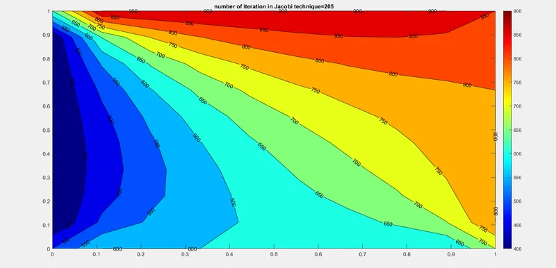
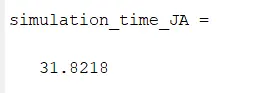
From the above plot , the number of iteration took to reach convergence is 205. The simulation took 31.8218 seconds.

The temparature at different positions can be obtained by placing the cursor at different co ordinates.

• For Gauss siedel iterative technique;

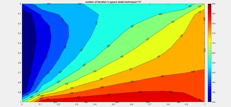
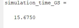
The Gauss siedl iterative technique took less time to converge. and less number of iterations. It took 111 number of iterations and 15.6750 seconds to simulate.

• For the SOR iterative technique

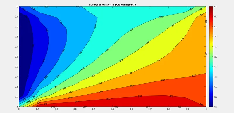
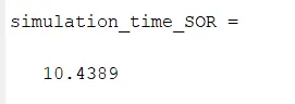
The SOR iterative technique took least number of iterations to converge. It took only 75 iterations to converge, and 10.4389 seconds time.

TRANSIENT HEAT CONDUCTION:

Transient heat conduction takes into account the time derivative term. The temperature field varies with respect to time also.

The equation stands as :

`(del^2T)/(delx^2) + (del^2T)/(dely^2) = (1/alpha)*(delT)/(delt)`--(5)

The left hand side of the above equation is the space derivative term, whereas the right hand side of the above equation is the time derivative term. since this involves the time derivative term , a time marching approach is taken in this case. Two approaches of solving the above equation can be taken up, namely explicit and implicit. In explicit approach , the discretization is done at the current time point i.e at n, whereas in the implicit approach, the discretization is done at the next time point i.e n+1. The explicit approach involves one equation with one unknown, so no iterative solvers are required to solve the equation. The implicit approach requires iterative solvers to solve.

From equation (5)

discretizing the LHS and he RHS :

`(T(i+1,j)-2*T(i,j)+T(i-1,j))/(deltax^2) +( T(i,j+1)-2*T(i,j)+T(i,j-1))/(deltay^2) = (1/alpha)*(T(n+1)-T(n))/(deltaT)`---(6)

here , T(n+1) is the value of T(i,j) at time point (n+1)

For explicit approach , the LHS is calculated at n and for implicit approach the LHS is calculated at (n+1)

MATLAB MODELLING:

Here the only additions are time step initialisation, the thermal diffusivity value is chosen , here it is of copper at 25 degree celsius. The time steps is considered. Inside the time loop , there is the space loop.

clear all
close all 
clc

%transient state 2D heat conduction
%explicit solution

%setting up the domain
l = 1; %length
h=1;   %breadth
nx=10; %number of nodes
ny =10;
x = linspace(0,l,nx); %creating the x array
y = linspace(0,h,ny);  %creating the y array
dx = 1/(nx-1);        %grit spacing
dy=1/(ny-1);

%setting the temperature profile
T=350*ones(nx,ny); %initial guess temperature
T(:,1)=400;        %boundary temprature(left)
T(:,nx)=800;       %boundary temperature(right)
T(1,:)=600;        %boundary temperature(top)
T(ny,:)=900;       %boundary temperature(bottom)
%edge refining by averaging
T(1,1)=500;
T(1,10)=700;
T(10,1)=650;
T(10,10)=850;

%creating a 2D array
[X,Y]=meshgrid(x,y);
%tolerance and error values ,time steps
dt = 1e-2;
tol=1e-4;
error=9e9;
%thermal diffusivity
alpha = 1.11*(10^-4); %for copper at 25 degree celsius. alpha = rho*c_p/k
%initialisng the T_old value to T , T_old is the previous value of
%temperature
T_old = T;

M = alpha*(dt/(dx^2));
N = alpha*(dt/(dy^2));
Z = 1-2*M-2*N;


tic

iter =1;
for nt = 1:1400
    while (error>tol)
        for i=2:nx-1
            for j = 2:ny-1
                T(i,j)=T_old(i,j)*Z+M*(T_old(i+1,j)+T_old(i-1,j))+N*(T_old(i,j+1)+T_old(i,j-1));
            end
        end
        error=max(max(abs(T_old-T)))
        iter = iter +1;
        T_old=T;
    end

    toc
    iter_explicit_time = toc


    figure(1)

    [A,B]=contourf(X,Y,T);
    set(gca,'YDIR','reverse')
    colorbar
    colormap(jet)
    clabel(A,B);
    text=sprintf('number of iteration in explicit technique=%d',iter);
    title(text)
end

OUTPUT:

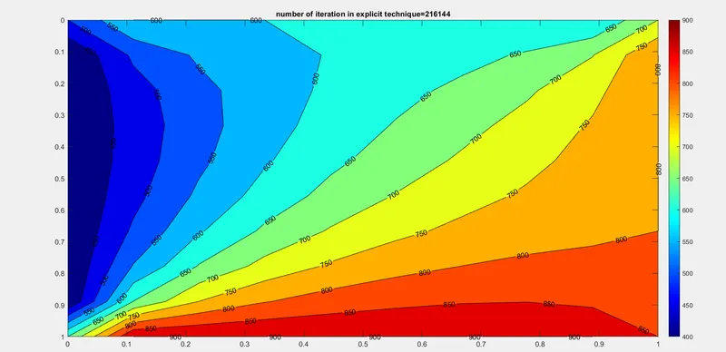
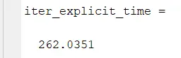
From the above plot , it is seen that the number of iterations are much higher than the steady state cases. It took nearly 216144 iterations to converge and 262.0351 seconds of time.

IMPLICIT APPROACH:

In the implicit approach, the parent equation becomes ;

`(T(i,j)^(n+1)-T(i,j)^n)/(deltaT)= alpha*((T(i-1,j)^(n+1)-2*T(i,j)^n+1+T(i+1,j)^n+1)/(deltax^2)+(T(i,j+1)^(n+1)-2*(T(i,j)^n+1)+T(i,j-1)^n+1)/(deltay^2)`---(7)

here there are more than one unknown and only one equation. Iterative solvers are used to solve the equation. Some modifications are done like the explicit approach for simplicity and ease of computing;

`M = alpha*(dT)/(dx^2)`

`N = alpha*(dT)/(dy^2)`

`Z = 1+2*M +2*N`

the term `alpha*(deltaT)/(deltax^2) and alpha*(deltaT)/(deltay^2)` are CFL numbers along the x space and y space . The CFL value for the entire analysis is `M+N`

The CFL value is important to determine and analyse the stabilty of the solution. This is discussed in later part of the report.

Namely Jacobi , Gauss Siedel and SOR iterative techniques are used to solve the problem .

MATLAB MODELLING:

• All other parameters are same like the previous ones , the time step is set to 0.001 , dt = 0.001
• Here T_prev is initialised to T ; and care is taken so that it is updated after the while loop. T_prev is the temperature value from the previous time point that is updated with every while loop.
• As it has a time derivative part , the space loop must be priovided inside the time loop.
• For SOR , the rlaxation factor is chosen as 1.11.

For the Jacobi iterative technique:

%transient2D heat conduction 
%implicit method
clear all
close all
clc

%setting up the domain
l = 1; %length
h=1;   %breadth
nx=10; %number of nodes
ny =10;
x = linspace(0,l,nx); %creating the x array
y = linspace(0,h,ny);  %creating the y array
dx = 1/(nx-1);        %grit spacing
dy=1/(ny-1);

T=350*ones(nx,ny); %initial guess temperature
T(:,1)=400;        %boundary temprature(left)
T(:,nx)=800;       %boundary temperature(right)
T(1,:)=600;        %boundary temperature(top)
T(ny,:)=900;       %boundary temperature(bottom)
%edge refining by averaging
T(1,1)=500;
T(1,10)=700;
T(10,1)=650;
T(10,10)=850;

%creating a 2D array
[X,Y]=meshgrid(x,y);
%tolerance and error values ,time steps
dt = 0.001;
tol=1e-4;
error=9e9;

%thermal diffusivity
alpha = 1.11; 
%initialisng the T_old value to T , T_old is the previous value of
%temperature
T_old = T;
T_previous = T;
M = alpha*(dt/(dx^2));
N = alpha*(dt/(dy^2));
CFL = M + N
Z = 1+2*M+2*N;
iterative_solver = input('Enter the choice:- 1)JA')
JA = 1;

tic
for nt = 1:1400%time loop
    if iterative_solver==1
        
        t1 = Z^(-1);
        t2 = M*t1;
        t3 = N*t1;
        error = 9e9;
        while error>tol
            %space loop
            for i = 2:nx-1
                for j = 2:ny-1
                    H = (T_old(i-1,j)+T_old(i+1,j));
                    V = (T_old(i,j+1)+T_old(i,j-1));
                    T(i,j) = t1*T_previous(i,j)+t2*H+t3*V;
                end
            end
            error = max(max(abs(T_old-T)));%since two dimensional 
            T_old = T;
            JA= JA +1;
        end
        T_previous = T;%updating the the previous time step value
    end
    toc;
    JA_iteretion_simulation_time = toc
    
    %plotting the results 
    figure(1)
    [A,B]=contourf(X,Y,T);
    set(gca,'YDIR','reverse')
    colorbar
    colormap(jet)
    clabel(A,B);
    text=sprintf('number of iteration in JA technique=%d',JA);
    title(text)
end
        

For the Gauss Siedel iterative technique:

%transient2D heat conduction 
%implicit method
clear all
close all
clc

%setting up the domain
l = 1; %length
h=1;   %breadth
nx=10; %number of nodes
ny =10;
x = linspace(0,l,nx); %creating the x array
y = linspace(0,h,ny);  %creating the y array
dx = 1/(nx-1);        %grit spacing
dy=1/(ny-1);

T=350*ones(nx,ny); %initial guess temperature
T(:,1)=400;        %boundary temprature(left)
T(:,nx)=800;       %boundary temperature(right)
T(1,:)=600;        %boundary temperature(top)
T(ny,:)=900;       %boundary temperature(bottom)
%edge refining by averaging
T(1,1)=500;
T(1,10)=700;
T(10,1)=650;
T(10,10)=850;

%creating a 2D array
[X,Y]=meshgrid(x,y);
%tolerance and error values ,time steps
dt = 0.001;
tol=1e-4;
error=9e9;

%thermal diffusivity
alpha = 1.11; 
%initialisng the T_old value to T , T_old is the previous value of
%temperature
T_old = T;
T_previous = T;
M = alpha*(dt/(dx^2));
N = alpha*(dt/(dy^2));
CFL = M + N
Z = 1+2*M+2*N;
iterative_solver = input('Enter the choice:- 1)GS')
GS = 1;

tic
for nt = 1:1400
    if iterative_solver==1
        
        t1 = Z^(-1);
        t2 = M*t1;
        t3 = N*t1;
        error = 9e9;
        while error>tol
            for i = 2:nx-1
                for j = 2:ny-1
                    H = (T(i-1,j)+T_old(i+1,j));
                    V = (T_old(i,j+1)+T(i,j-1));
                    T(i,j) = t1*T_previous(i,j)+t2*H+t3*V;
                end
            end
            error = max(max(abs(T_old-T)));
            T_old = T;
            GS = GS +1;
        end
        T_previous = T;
    end
    toc;
    GS_iteretion_simulation_time = toc
    
    %plotting the results 
    figure(1)
    [A,B]=contourf(X,Y,T);
    set(gca,'YDIR','reverse')
    colorbar
    colormap(jet)
    clabel(A,B);
    text=sprintf('number of iteration in GS technique=%d',GS);
    title(text)
end
        

For SOR technique:

%transient2D heat conduction 
%implicit method
clear all
close all
clc

%setting up the domain
l = 1; %length
h=1;   %breadth
nx=10; %number of nodes
ny =10;
x = linspace(0,l,nx); %creating the x array
y = linspace(0,h,ny);  %creating the y array
dx = 1/(nx-1);        %grit spacing
dy=1/(ny-1);

T=350*ones(nx,ny); %initial guess temperature
T(:,1)=400;        %boundary temprature(left)
T(:,nx)=800;       %boundary temperature(right)
T(1,:)=600;        %boundary temperature(top)
T(ny,:)=900;       %boundary temperature(bottom)
%edge refining by averaging
T(1,1)=500;
T(1,10)=700;
T(10,1)=650;
T(10,10)=850;

%creating a 2D array
[X,Y]=meshgrid(x,y);
%tolerance and error values ,time steps
dt = 0.001;
tol=1e-4;
error=9e9;
beta = 1.12; %relaxation factor for the SOR
%thermal diffusivity
alpha = 1.11; 
%initialisng the T_old value to T , T_old is the previous value of
%temperature
T_old = T;
T_previous = T;
M = alpha*(dt/(dx^2));
N = alpha*(dt/(dy^2));
CFL = M + N
Z = 1+2*M+2*N;
iterative_solver = input('Enter the choice:- 1)SOR')
SOR = 1;

tic
for nt = 1:1400
    if iterative_solver==1
        
        t1 = Z^(-1);
        t2 = M*t1;
        t3 = N*t1;
        error = 9e9;
        while error>tol
            for i = 2:nx-1
                for j = 2:ny-1
                    H = (T(i-1,j)+T_old(i+1,j));
                    V = (T_old(i,j+1)+T(i,j-1));
                    T(i,j) = (1-beta)*T_old(i,j)+beta*(t1*T_previous(i,j)+t2*H+t3*V);
                end
            end
            error = max(max(abs(T_old-T)));
            T_old = T;
            SOR = SOR +1;
        end
        T_previous = T;
    end
    toc;
    SOR_iteretion_simulation_time = toc
    
    %plotting the results 
    figure(1)
    [A,B]=contourf(X,Y,T);
    set(gca,'YDIR','reverse')
    colorbar
    colormap(jet)
    clabel(A,B);
    text=sprintf('number of iteration in SOR technique=%d',SOR);
    title(text)
end
        

OUTPUT:

Jacobi Iteration:

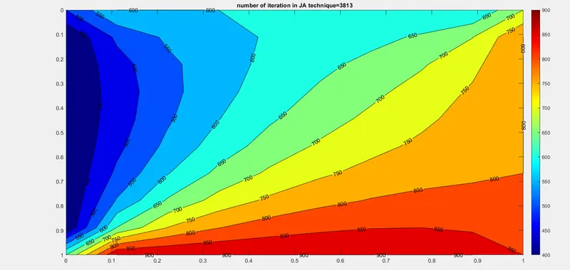
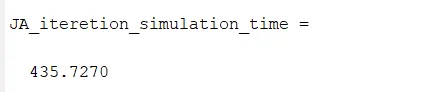
The CFL value came to be as 0.17 , which by the criterion of stability is stable. The time taken to complete the itertion is 435.7270 seconds. The Jacobi iterative technique took 3813 iterations to converge.

Gauss Siedel iteration:

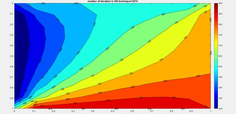
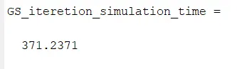
The Gauss siedel iterative technique took 3274 iterations to come at convergence at 371.2371 seconds

SOR iteration:

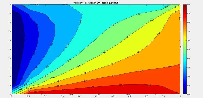
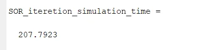
The SOR iterative technique took least amount of time to converge. The number of iterations taken to converge is also lowest. It took only 2885 iterations.

INFERENCE :

• Matlab modelling of a two dimensional heat transfer equation for both transient and steady state is done and the temperature distribution is visualised in a selected domain.
• The convergence rate of SOR technique is highest and it takes least number of iterations to converge at the solution
• The Stability criterion is governed by the CFL number. If CFL number is less than or equal to 0.5 , the solution is stable. The CFL number is obtained by summing the CFL nuber along the x space and y space ,
• CFL|x = `alpha*(dT)/(dx^2)` and CFL|y= `alpha*(dT)/(dx^2)`
• The relaxation factor in case of SOR technique needs to be chosen carefully. If it is chosen below 1, it is called under relaxed. if it is chosen more than 1 , it is called over relaxed. However , if chosen as 2 or near 2, the iteration overshoots . it misses the next node of the current node .
• By comparing the time taken to converge , SOR technique converges fastest . next is the Gauss siedel technique , Jacobi iterative technique converges slowest. Number of iterations taken for convergence is highest for Jacobi technique, lowest for SOR technique, and in between lies the Gauss Siedl technique.
• The Explicit approach took more iterations to converge than the implicit approach .