Week 5 - Genetic Algorithm
Aim:
a) To write code to optimize the stalagmite function, and to find the global maxima of the function.
b) Plot graphs for all 3 case studies.
Theory:
Stalagmite Optimization Function
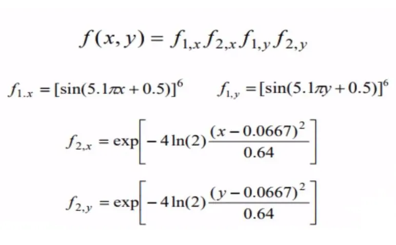
Stalagmite Functions are mathematical functions, used to determine global and local maxima and minima. The function is defined as shown below.
Genetic Algorithm
The Genetic Algorithm is one of the optimization processes that uses the principle of genetics and natural selection to obtain an optimal and near-optimal solution. The following are the steps involved in an optimization technique.
Step 1- Population Initialization
The optimization process begins with an initialization step where the population size is decided. Population size helps in deciding the accuracy of the solution because a higher size gives more combinations and thus provides more accurate results. In simple words, GA operations are performed using a sample set of data points known as population size.
Step 2- Selection
The initialization step is followed by a selection process. In this process, parents are randomly selected from the sample population size. The purpose is to select highly fit individuals for the next generation. Highly fit individuals of a function are determined by computing its fitness value.
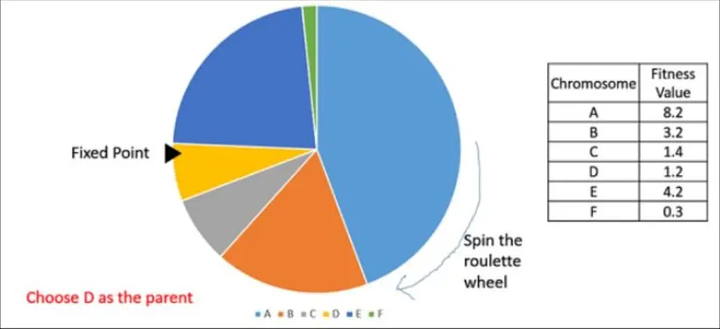
fig.1 Roulette wheel selection for the fittest individual
The computed fitness value of a given function for different data points is represented in the form of a pie chart or using a roulette wheel (Roulette wheel selection shown in the above figure). To select the fittest individual roulette wheel is rotated. The fittest value has the highest probability to become a parent as it covers a greater area in a roulette wheel. It helps to select the best individuals for transmitting their best characteristics to future generations.
Step-3 Cross-Over
The process of producing children from two parents by interchanging their genes is known as cross-over.
Step-4 Mutation
Mutation is carried out to create genetic diversity for the next generation. Mutation avoids convergence to happen soon. It creates dissimilarity among the children.
The process gets repeated again and again by selecting different parents until the fittest individual is found. The fitness of a function is a measure of the goodness of a solution or how close the solution is to the optimal solution.
ga Syntax
x=ga(fun,nvars,A,b,Aeq,beq,lb,ub,nonlcon,intcon,options)
fun- function A - Linear inequality constraints(real matrix)
nvars- no. of variables b - Linear inequality constraints(real vector)
Aeq - Linear equality constraints(real matrix) beq - Linear equality matrix(real vector)
lb - lower bounds ub - upper bounds
nonlcon- non-linearity constraints intcon - integer constraints
options - optimisation options
Program Code for stalagmite function
The stalagmite function is coded as per the equations given in the introduction.
function[fxy] = stalagmite11(input_v)

x = input_v(1);
y = input_v(2);


c1 = 5.1*pi;

f_1x = sin((c1*x)+(0.5)).^6;

f_1y = sin((c1*y)+(0.5)).^6;

c2 = -4*log(2)./(0.64);

f_2x = exp(c2*(x-0.0667).^2);

f_2y = exp(c2*(y-0.0667).^2);

fxy = -f_1x*f_2x*f_1y*f_2y;
end
Program code for genetic algorithm using stalagmite function
clear all
close all
clc

% search space definition for ga function

x = linspace(0,0.6,150);
y = linspace(0,0.6, 150);

[xx,yy] = meshgrid(x,y); % 2-D Array using meshgrid

for i= 1:length(xx)
    for j= 1:length(yy)
        input_v(1) = xx(i,j);
        input_v(2) = yy(i,j);
        f(i,j) = stalagmite11(input_v); %calling stalagmite function
    end
end


% Case Study_1: No boundary limits

num_cases = 50;  % number of iterations
tic
for i = 1:num_cases

    [outputs, fopt(i)] = ga(@stalagmite11,2);
    xopt(i) = outputs(1);
    yopt(i) = outputs(2);

end
study_time1 = toc % time taken

figure(1)
subplot(2,1,1)
surfc(xx,yy,-f)
shading interp
hold on
plot3(xopt,yopt,-fopt,'marker','o','markersize',5,'markerfacecolor','r')
subplot(2,1,2)
plot(-fopt)
xlabel('Iterations')
ylabel('Func Maximum')

% Case Study_2: Boundary Conditions Defined

tic
for i = 1:num_cases

    [outputs, fopt(i)] = ga(@stalagmite11,2,[],[],[],[],[0;0],[1;1]);
    xopt(i) = outputs(1);
    yopt(i) = outputs(2);

end
study_time2 = toc

figure(2)
subplot(2,1,1)
surfc(xx,yy,-f)
shading interp
hold on
plot3(xopt,yopt,-fopt,'marker','o','markersize',5,'markerfacecolor','r')
subplot(2,1,2)
plot(-fopt)
xlabel('Iterations')
ylabel('Func Maximum')

% Case Study_3: Population Size Defined

options = optimoptions('ga');
options = optimoptions(options,'populationsize',350);

tic
for i = 1:num_cases

    [outputs, fopt(i)] = ga(@stalagmite11,2,[],[],[],[],[0;0],[1;1],[],[],options);
    xopt(i) = outputs(1);
    yopt(i) = outputs(2);

end
study_time3 = toc

figure(3)
subplot(2,1,1)
surfc(xx,yy,-f)
shading interp
hold on
plot3(xopt,yopt,-fopt,'marker','o','markersize',5,'markerfacecolor','r')
subplot(2,1,2)
plot(-fopt)
xlabel('Iterations')
ylabel('Func Maximum')
Code Explanation
a) The script begins with clear all, close all, clc that clears the workspace data closes the figure windows and clears the command window.
b) 'x' & 'y' are input arrays of equal intervals between 0 & 150 created using linspace.
c) The two input arrays are further used to create a 2- D array using the meshgrid command.
d) To evaluate the stalagmite function, two for loops 'i' and 'j' are utilized. Inputs for the stalagmite function get stored in a variable 'input_v'.
e) A stalagmite function is prepared after which the output is utilized to study three different cases of ga.
f) Study 1 happens without setting the boundary limits with the number of iterations set to 50. 'outputs and 'fopt' are the two output variables of a GA function. 'outputs' give that input 'x' and 'y' which results in optimum 'fopt'. For this study, ga syntax calls the stalagmite function and defines the number of variables as 2.
g) Time taken for the optimization process is recorded as 'study_time'.
h) ga function evaluates the minimum value. Hence to identify the global maxima of the stalagmite function, the values stored in 'fopt' is multiplied with '-1'. Thus the minimum value identified by ga becomes the global maxima of a stalagmite.
i) Then the results are plotted in graphs. The 'subplot' command is used to plot multiple plots in the same figure window. The function in the loop is plotted using 'surfc' command. To obtain a smooth plot without gridlines, 'shading interp' command is used. 'plot3' command is used to plot 3-D points at 'xopt', 'yopt', 'fopt' using red colored 'o' marker of size 5. Also, 'fopt' is plotted separately for 50 iterations to find the maximum value of the function.
j) In study two, boundary conditions are defined to restrict the variation in results in study 1 each time we run the program. An upper and lower bound is defined additionally in the ga syntax. The remaining code is similar to study 1.
k) In the final study, population size is defined to get a more accurate result.Therefore to consider the population size, the syntax "options = optimoptions('solver name','name',value)" with 'name' 'populationsize' and 'value' set to 350. The syntax for ga contains additional 'options' terms and the code remains the same as in study 1.
Results & Graphs
Case _Study - 1
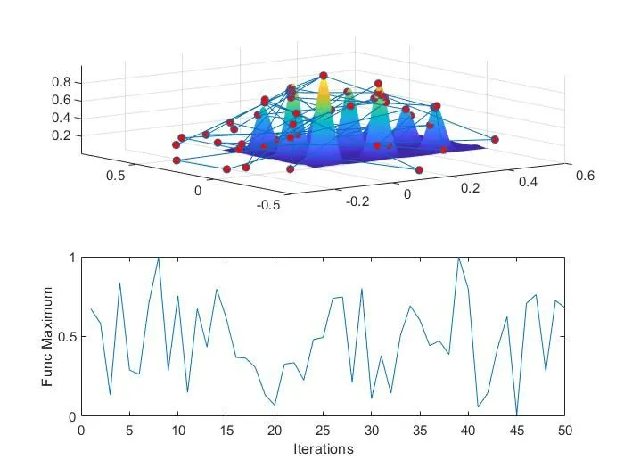
In this graph, ga generates a new optimum value in every single iteration. The maximum value of the function varies continuously between 0 to 1. Since the final value changes in each iteration, the solution is not reliable. Therefore a second case study is done with upper and lower bounds specified.
Statistical Behaviour (Unbound Case)
Case_Study - 2
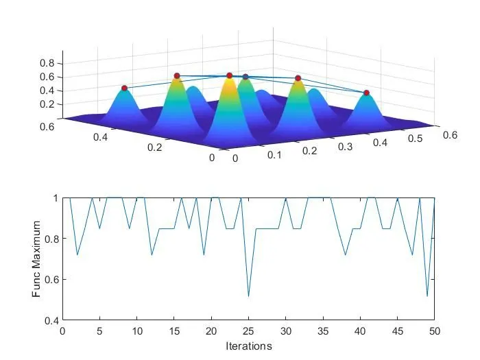
In this study, upper and lower bounds are specified in the ga syntax. As a result, the number of red dots in the plot reduced compared to case study 1. The function maximum is in the range of 0.5 to 1 which means that the variation in the optimum value in each iteration started to converge.
Bound Case (Upper and Lower Bounds Specified)
Case_Study- 3
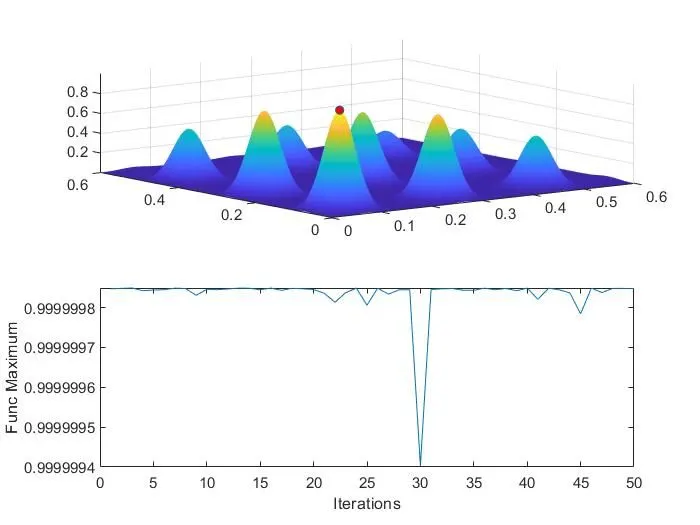
In this case, the population size is increased to 350 to refine the result further. This has produced a reliable result with the function maximum closer to 1 in each iteration. The global maxima are at x=0.0668 and y= 0.0668.
Statistical Behaviour with Population Size Defined
Workspace
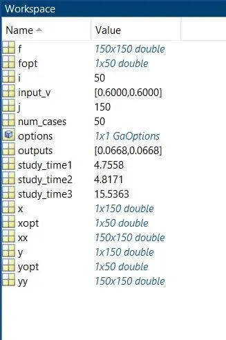
The global maxima are obtained at x=0.0668 and y=0.0668. The study time of each case can be found in the workspace.
References
a) https://skill-lync.com/knowledgebase/genetic-algorithm-explained