Week 3 - Solving second order ODEs

Aim:

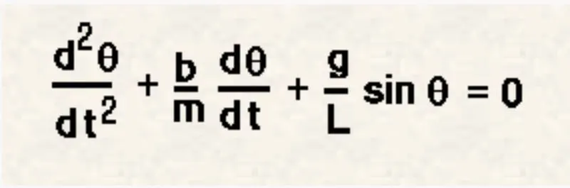
       a) Write a program to solve the below second order differential equation.

        

       b) Write a program to simulate pendulum motion.

Theory:

 a) The second-order differential equation, represents the damped motion of a simple pendulum.

 b)  The transient behaviour of a system can be represented with the help of an ODE.

 c) Newton's second law of motion " The rate of change of momentum of a body over time is directly proportional to the force applied and occurs in the same direction as the applied force."

                                                        F= m*a

d) The pendulum motion is an example of Newton's second law of motion, and the second-order differential equation represents the position of the bob with respect to time.

Procedure: Program to solve a second-order differential equation

 a) The second-order differential equation is converted to a first-order differential equation for the ease of function operation.

Program Code

clear all
close all
clc

% Program to solve the ODE that represents the damped motion of a simple pendulum

% inputs
l = 1;     % length of the pendulum in m
m = 1;     % mass of the ball in kg
b = 0.05;  % damping coefficient
g = 9.81;  %  m/s^2

% initial conditions
theta_0 = [0;3]; % angular displacement in radian and angular velocity in rad/sec
t_span = linspace(0,20,300); % time span

% solving the ODE
[t,results] =ode45(@(t,theta)ode_function(t,theta,b,g,l,m),t_span,theta_0);


% plots

figure(1) % plot representing the damping motion 
plot(t,results(:,1))  % displacement of bob in radians
hold on
plot(t,results(:,2))  % velocity of bob in rad/sec

xlabel('time')
ylabel('velocity&displacement')

Displacement = results(:,1);

% Program to simulate pendulum motion

ct=1;
for i= 1:length(Displacement) % for loop for the pendulum motion
    
    theta_1= Displacement(i);
    
    x0 = 0;
    y0 = 0;
    x1 =  l*sin(theta_1); 
    y1 = -l*cos(theta_1); % Negative Y axis


figure(2) % pendulum motion

plot([x0 x1],[y0 y1],'linewidth',0.75)
hold on

plot(x1,y1,'O','markerfacecolor','r','markersize',8)
hold off

 axis([-2 2 -1.2 0.2]) 
   
 pause(0.01) % Each frame gets paused for a given period of time
 
 M(ct) = getframe(gcf); % An array of plots assigned to 'M'
 
 ct = ct+1;

end

movie(M) % creating a movie out of all frames assigned to 'M'
videofile = VideoWriter('pendulum_motion.avi','Uncompressed AVI');
open(videofile)
writeVideo(videofile,M)
close(videofile)

 Step-wise explanation of the code

a) The input for the program to solve the ODE such as length of the pendulum(l), the mass of the bob(m), coefficient of damping(b), acceleration due to gravity(g) are applied to the corresponding variables.

b) Initial conditions such as angular displacement and angular velocity are applied to simulate pendulum motion for a span of 20 seconds.

c) The second-order differential equation is solved using the function 'ode45', which takes 3 inputs, the function to be integrated, the time span and the initial conditions.

d) The function to be integrated is defined separately as 'ode_function', and the code for the function is shown below.

function [dtheta_dt]= ode_function(t,theta,b,g,l,m)

theta1=theta(1);
theta2=theta(2);
dtheta1_dt = theta2;
dtheta2_dt = (-b/m)*theta2-(g/l)*sin(theta1);
dtheta_dt = [dtheta1_dt;dtheta2_dt];
end

e) The function 'ode_funtion' is defined separately, and within the function, the second-order differential equation is reduced to two first-order differential equations which are finally solved using the function 'ode45'.

f) Finally, the displacement and velocity for the damped motion of the pendulum for the given time span are evaluated and plotted graphically.

                                                  

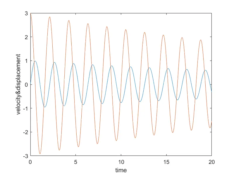
                                                                                             The damped motion of a simple pendulum

g) To simulate the motion of simple pendulum a for loop with the length equivalent to the length of the results is applied.

h) Value of displacement is taken individually and the position of bob is computed with the help of trigonometric functions sin and cos.

i) The position from where the pendulum is hung is taken to be the origin. Marker command is used to represent the bob and to colour the bob. 

j) A proper axis is selected to view the motion of the pendulum. Each frame is paused for a given period of time.

k) Each frame is added to an array 'M', which further used to create a movie or video.

Learning Outcome:

a) Learned to solve a higher order differential equation.

b) Learned to simplify a higher-order derivative to a series of lower-order derivatives.

c) Learned to simulate a damped motion.

Results:

a) ODE solved successfully.

b) Damped pendulum motion simulated successfully.

c) Link for the animated video

 https://drive.google.com/file/d/1Rrf7AZjYrulMBSVL5LjQ5L-RDOlsUR-2/view?usp=sharing