Challenge

Week 5 - Genetic Algorithm

AAnish Kumar Sharma22 Sept 2022

MATLAB

AIM:

Write a code in MATLAB to optimise the stalagmite function and find the global maxima of the function.
Clearly expalin the concept of genetic algorithm in your own words and also explain the syntax for ga in MATLAB in your report.
Make sure that your code gives the same output, even if it is made to run several times.
Plot graphs for all 3 studies and for F maximum vs no. of iterations. Title and axes labels are a must, legends could be shown if necessary.

SOLUTION:

Programming Language: MATLAB

Code:-

Function Code -

function

f = stalagmite(input_vector)

fx = (sin(5.1*pi*input_vector(1)+0.5))^6;

fy = (sin(5.1*pi*input_vector(2)+0.5))^6;

fxx = exp((-4*log(2)*(((input_vector(1)-0.0667)^2)/0.64)));

fyy = exp((-4*log(2)*(((input_vector(2)-0.0667)^2)/0.64)));

f = -(fx*fy*fxx*fyy);

end

Main Code -

clear

clc

%1) Input

x = linspace(0,0.6,200);

y = linspace(0,0.6,200);

num_cases=50;

%2) use of meshgrid command

[xx,yy] = meshgrid(x,y);

%3) Evaluating objective function by using mested loop

for i = 1:length(xx)

for j = 1:length(yy)

input_vector(1) = xx(i,j);

input_vector(2) = yy(i,j);

f(i,j) = stalagmite(input_vector);

end

% plot the results in the form of surface plot

figure(1)

surf(xx,yy,-f)

shading interp

% performing GA study

%1) Unbounding study

tic

for i=1:num_cases

[input,fopt(i)] = ga(@stalagmite,2);

xopt(i) = input(1);

yopt(i) = input(2);

end

time_study1 = toc;

figure(2)

subplot(2,1,1)

hold on

surfc(x,y,-f)

shading interp

plot3(xopt,yopt,-fopt,'Marker','o','markersize',5,'MarkerFaceColor','r')

title('Unbounded Input')

%Figure(2)

subplot(2,1,2)

plot(-fopt)

xlabel('Iteration')

ylabel('Function Maximum')

%2) Bounded study

tic

for i=1:num_cases

[input2,fopt2(i)] = ga(@stalagmite,2,[],[],[],[],[0,0],[0.6,0.6]);

xopt2(i) = input2(1);

yopt2(i) = input2(2);

end

time_study2 = toc;

figure(3)

subplot(2,1,1)

hold on

surfc(x,y,-f)

shading interp

plot3 (xopt2,yopt2,-fopt2,'Marker','o','markersize',5,'MarkerFaceColor','r')

title('Bounded Input')

%Figure(2)

subplot(2,1,2)

plot(-fopt2)

xlabel('Iteration')

ylabel('Function Maximum')

%3) Case_Study 3: Maximising the population size to optimize the result

options = optimoptions ('ga');

options = optimoptions (options,'PopulationSize',500);

tic

for i=1:num_cases

[input3,fopt3(i)] = ga(@stalagmite,2,[],[],[],[],[0,0],[0.6,0.6],[],[],options);

xopt3(i) = input3(1);

yopt3(i) = input3(2);

end

time_study3 = toc;

figure(4)

subplot(2,1,1)

hold on

surfc(x,y,-f)

shading interp

plot3 (xopt3,yopt3,-fopt3,'Marker','o','markersize',5,'MarkerFaceColor','r')

title('Bounded Input')

%Figure(2)

subplot(2,1,2)

plot(-fopt3)

xlabel('Iteration')

ylabel('Function Maximum')

Code Explanation:-

Before writing the code, it's important to start with clear all, close all and clc commands since

Clear all - removes data from the workspace, freeing up system memory

Close all- deletes the current figure or the specified figure

clc - clears all input and output from the Command Window display, giving you a "clean screen"

firstly we create Function code to Optimize stalagmite Function

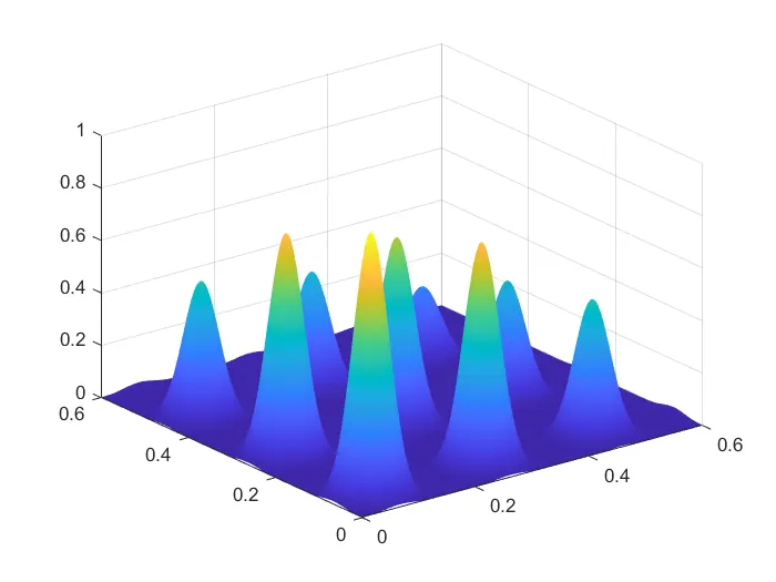
Then in main code we insert the inputs that are known such as the values of x,y, and num_cases then using Meshgrid command we creat 2D array from 1D array of x and y to xx and yy then , we evaluate objective function by using nested loop in which we introduces the stalagmite function to the main code, then plot the resulyt in thr form of surface plot as we know stalagmite function gives -ve values so me add- sign to reverse that so that we can get +ve values.

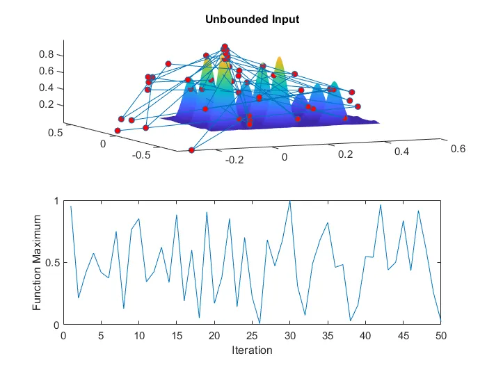
UNBOUNDED STUDY:- Here we create a FOR loop because it will be help ful to cover the 2D inputs, In this loop for every point in the xy plane stalagmite function will be called to calculate the value of 'f'. Here in GA syntax the lower and upper bounds are not defined so the results are not accurate .

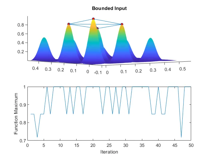
BOUNDED STUDY:- We create a FOR loop simillar to UNBOUNDED STUDY but our GA syntax will change because in this study boundaries is provided (ga(@stalagmite,2,[],[],[],[],[0,0],[0.6,0.6]) because of these boundary results are confined by which answer is more accurate.

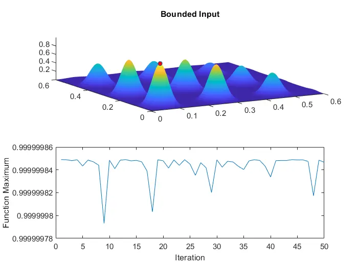
BOUNDED STUDY(Maximising the population size):- In this study FOR loop is created with optimized boundaries (ga(@stalagmite,2,[],[],[],[],[0,0],[0.6,0.6],[],[],options), these boundaries will help in narrowing the answer or we can say optimize the solution tho tha maximum

USE OF THE FOLLOWING FUNCTIONS USED WHILE PROGRAMMING

FOR LOOP- For loop is used here for the iteration of the theta values from 0 to 90 degrees I is used as the outer loop and J is used as the inner loop ,i is used for the movement of the link 1 and J is used for the movement of link 2.

Plot - The plot command is used to plot the graphs of the coordinates provided.

GA - ga(fun,nvars,A,b,Aeq,beq,lb,ub,nonlcon,intcon,options) requires that the variables listed in intcon take integer values.

Tic - Tok - tic works with the toc function to measure elapsed time. The tic function records the current time, and the toc function uses the recorded value to calculate the elapsed time.

Subplot - subplot(m,n,p) divides the current figure into an m-by-n grid and creates axes in the position specified by p. MATLAB^® numbers subplot positions by row. The first subplot is the first column of the first row, the second subplot is the second column of the first row, and so on. If axes exist in the specified position, then this command makes the axes the current axes.

Shading - shading interp varies the color in each line segment and face by interpolating the colormap index or true color value across the line or face.

Surf - surf(X,Y,Z) creates a three-dimensional surface plot, which is a three-dimensional surface that has solid edge colors and solid face colors. The function plots the values in matrix Z as heights above a grid in the x-y plane defined by X and Y. The color of the surface varies according to the heights specified by Z.

Xlabel - xlabel(txt) labels the x-axis of the current axes or standalone visualization. Reissuing the xlabel command replaces the old label with the new label.

Ylabel - ylabel(txt) labels the y-axis of the current axes or standalone visualization. Reissuing the ylabel command causes the new label to replace the old label.

Title - title(titletext) adds the specified title to the current axes or standalone visualization. Reissuing the title command causes the new title to replace the old title.

Figure - figure creates a new figure window using default property values. The resulting figure is the current figure

Hold - hold on retains plots in the current axes so that new plots added to the axes do not delete existing plots. New plots use the next colors and line styles based on the ColorOrder and LineStyleOrder properties of the axes. MATLAB^® adjusts axes limits, tick marks, and tick labels to display the full range of data. If axes do not exist, then the hold command creates them.

Optimotions - options = optimoptions(SolverName,Name,Value) returns options with specified parameters set using one or more name-value pair arguments.

Week 5 - Genetic Algorithm

Ship work like this
in your own course.

Talk to a career counsellor

Ship work like thisin your own course.

Talk to a career counsellor

Ship work like this
in your own course.