Week 4.1 - Solving second order ODEs
AIM: Write a program in MATLAB\Octave that will simulate the pendulum motion.
DESCRIPTION: In Engineering, ODE is used to describe the transient behavior of a system. A simple example is a pendulum.
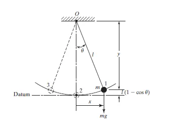
Figure1: A simple pendulum.
A simple pendulum is one that can be considered to be a point mass suspended from a string or rod of negligible mass. It is a resonant system with a single resonant frequency.
GOVERNING EQUATIONS: The way the pendulum moves depends on Newton's second law. When this law is written down, we get a second order Ordinary Differential Equation that describes the position of the "ball" w.r.t time.
In the above equation,
g = gravity in m/s2,
L = length of the pendulum in m,
m = mass of the ball in kg,
b=damping coefficient.
Write a program in Matlab\Octave that will simulate the pendulum motion, just like the one shown in the start of this challenge.
Given Values:-
L=1 metre,
m=1 kg,
b=0.05.
g=9.81 m/s2.
Simulate the motion between 0-20 sec, for angular displacement=0,angular velocity=3 rad/sec at time t=0.
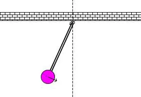
When you do this you will get the position of the pendulum as a function of time. Use this information to animate the motion of the pendulum, as shown in the below figure.
CODE
Function Code -
Main code -
Code Explanation:-
Before writing the code, it's important to start with clear all, close all and clc commands since
Clear all - removes data from the workspace, freeing up system memory
Close all- deletes the current figure or the specified figure
clc - clears all input and output from the Command Window display, giving you a "clean screen
Function Code - In this we create a function code for splitting the second order derivation into two parts dtheta1_dt and dtheta2_dt and combine those two into one as dtheta_dt
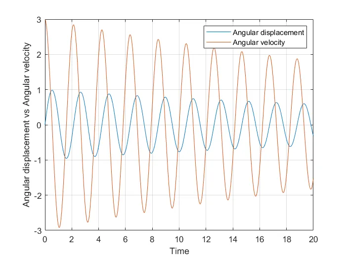
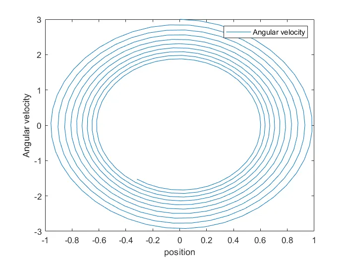
Main Code - in main code we input all the given values, then the initial conditions are coded into the code. In second step we create an array for given time using 'Linspace' command then we create Solver code in thirsd stepusing 'ODE45' code then we plot all of our findingwe plot 2 figures.
The final step of the code is to create a movie of the animation of the Pendulum, so the movie command was used. The VideoWriter command was used to assign the video format, for this project .avi was used as the format. The open command was used to open the video. writevideo command was used to write the video with plot frames. Finally, the close command was used to close the video file.
USE OF THE FOLLOWING FUNCTIONS USED WHILE PROGRAMMING
FOR LOOP- For loop is used here for the iteration of the theta values from 0 to 90 degrees I is used as the outer loop and J is used as the inner loop ,i is used for the movement of the link 1 and J is used for the movement of link 2.
PAUSE - We have paused the code so that the process can be visualised more clearly .
Ct-Ct is used for saving the frames in order to create a movie of the frames
Getframe-Similarly getframe is used to capture the frame and then by fast movement of those frames it can be converted into a movie
Movie -Movie command is used to create a movie of the frames captured .
VideoWriter -It is to create a Video file of the movie created and save in the pc hard disc.
Plot - The plot command is used to plot the graphs of the coordinates provided.
Axis- The axis command is used to create the axis upon which we are going to plot the coordinates.
Linspace-The linspace command is useful in creating an array of values specified by the user.
RESULT:- https://youtu.be/VhCkijFMlVg